Attention专场——(2)Self-Attention 代码解析
文章目录
- 1. 参考资料
- 2. 模型架构
- 2.1 Encoder and Decoder Stacks
- 2.1.1 通用类
- 2.1.1.1 层的复制函数
- 2.1.1.2 LayerNorm类
- 2.1.1.3 sublayer之间的连接方式
- 2.1.4 Encoder
- 2.1.4.1 EncodeLayer类
- 2.1.5 Decoder
- 2.3 Attention
- 2.3.1 Attention方式
- 2.3.2 multi-head attention
- 2.4 在模型中使用Attention
- 2.5 Position-wise Feed-Forward Networks
- 2.6 Embedding and Softmax
- 2.7 Position Encoding
- 3 Full Model
- 4. Training
- 4.1 Batches and Masking
- 4.2 training loop
- 4.3 Training Data and Batching
- 4.4 优化函数
- 4.5 Regularization
- 参考链接
- 5. 总结
1. 参考资料
- Attention Is All You Need - NIPS 2017: 5998-6008 - 论文链接
- transformer原理参考文章
- transformer中文讲解视频(简单)
- transformer中文讲解视频(进阶)
- 哈佛大学的ptorch版transformer代码实现
- 自注意力与位置编码
- 汉语自然语言处理-从零解读碾压循环神经网络的transformer模型(一)
- 汉语自然语言处理-BERT的解读语言模型预训练与实践应用-transformer模型(二)
- 标签平滑简介
- postition encoding
2. 模型架构
编码器将输入序列 ( x 1 , x 2 , . . . , x n ) (x_1, x_2, ..., x_n) (x1,x2,...,xn)映射成序列 z = ( z 1 , . . . , z n ) \bold{z}=(z_1, ..., z_n) z=(z1,...,zn)。要考虑给定 z \bold{z} z的情况下,解码器产生序列 ( y 1 , . . . , y m ) (y_1, ..., y_m) (y1,...,ym)的情况,每一步的输出不仅要考虑当前的输入,还要考虑上一步的输出。
因此,定义结构如下:
class EncoderDecoder(nn.Module):
    """
    A standard Encoder-Decoder architecture. Base for this and many
    other models.
    """
    def __init__(self, encoder, decoder, src_embed, tgt_embed, generator):
        super(EncoderDecoder, self).__init__()
        self.encoder = encoder
        self.decoder = decoder
        self.src_embed = src_embed
        self.tgt_embed = tgt_embed
        self.generator = generator

    def forward(self, src, tgt, src_mask, tgt_mask):
        "Take in and process masked src and target sequences."
        return self.decode(self.encode(src, src_mask), src_mask,
                            tgt, tgt_mask)

    def encode(self, src, src_mask):
        return self.encoder(self.src_embed(src), src_mask)

    def decode(self, memory, src_mask, tgt, tgt_mask):
        return self.decoder(self.tgt_embed(tgt), memory, src_mask, tgt_mask)
class Generator(nn.Module):
    "Define standard linear + softmax generation step."
    def __init__(self, d_model, vocab):
        super(Generator, self).__init__()
        self.proj = nn.Linear(d_model, vocab)

    def forward(self, x):
        return F.log_softmax(self.proj(x), dim=-1)
2.1 Encoder and Decoder Stacks

2.1.1 通用类
2.1.1.1 层的复制函数
# 定义一个层复制函数,将每一层的结构执行深拷贝,并返回list形式
def clones(module, N):
    "Produce N identical layers."
    return nn.ModuleList([copy.deepcopy(module) for _ in range(N)])
2.1.1.2 LayerNorm类
# 定义layer的正则化类,与batchsize同的是:
# batch_size的目的是将一个epoch中的数据标准化,标准化的是不同样本中的同一特征。
# layer_size的目的是将一个样本中的数据标准化。
class LayerNorm(nn.Module):
    "Construct a layernorm module (See citation for details)."
    def __init__(self, features, eps=1e-6):
        super(LayerNorm, self).__init__()
        self.a_2 = nn.Parameter(torch.ones(features))
        self.b_2 = nn.Parameter(torch.zeros(features))
        self.eps = eps

    def forward(self, x):
        mean = x.mean(-1, keepdim=True)
        std = x.std(-1, keepdim=True)
        return self.a_2 * (x - mean) / (std + self.eps) + self.b_2
2.1.1.3 sublayer之间的连接方式
# 定义残差连接层。
# 这里的forward函数代表的意思是:
# 如果该层没有跳过的话,那么返回就是该层的计算结果
# 如果该层被drop了,那么直接把该层的输入作为输出
class SublayerConnection(nn.Module):
    """
    A residual connection followed by a layer norm.
    Note for code simplicity the norm is first as opposed to last.
    """
    def __init__(self, size, dropout):
        super(SublayerConnection, self).__init__()
        self.norm = LayerNorm(size)
        # 设置丢弃的概率
        self.dropout = nn.Dropout(dropout)

    def forward(self, x, sublayer):
        "Apply residual connection to any sublayer with the same size."
        return x + self.dropout(sublayer(self.norm(x)))
2.1.4 Encoder
encoder 由6个完全一样的层叠加而成。
# 定义encoder的前向传播计算方法,重复N次
class Encoder(nn.Module):
    "Core encoder is a stack of N layers"
    def __init__(self, layer, N):
        super(Encoder, self).__init__()
        self.layers = clones(layer, N)
        self.norm = LayerNorm(layer.size)

    def forward(self, x, mask):
        "Pass the input (and mask) through each layer in turn."
        for layer in self.layers:
            x = layer(x, mask)
        return self.norm(x)
该层中add 的部分主要是将multi-head attention的output与multi-head attention的input相加。然后在执行layer的norm操作。
2.1.4.1 EncodeLayer类
Each layer has two sub-layers. The first is a multi-head self-attention mechanism, and the second is a simple, position-wise fully connected feed- forward network.
每一个encoder层中都有两个子层,一个是多头注意力机制,一个是位置的信息。

class EncoderLayer(nn.Module):
    "Encoder is made up of self-attn and feed forward (defined below)"
    def __init__(self, size, self_attn, feed_forward, dropout):
        super(EncoderLayer, self).__init__()
        # attention机制
        self.self_attn = self_attn
        # 全连接的位置信息
        self.feed_forward = feed_forward
        self.sublayer = clones(SublayerConnection(size, dropout), 2)
        self.size = size

    def forward(self, x, mask):
        "Follow Figure 1 (left) for connections."
        x = self.sublayer[0](x, lambda x: self.self_attn(x, x, x, mask))
        return self.sublayer[1](x, self.feed_forward)
至此,输出的结果就变成了LayerNorm(x+Sublayer(x))。
2.1.5 Decoder
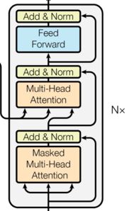
和encoder层一样,decoder层也由N个一样的层组成。
class Decoder(nn.Module):
    "Generic N layer decoder with masking."
    def __init__(self, layer, N):
        super(Decoder, self).__init__()
        self.layers = clones(layer, N)
        self.norm = LayerNorm(layer.size)

    def forward(self, x, memory, src_mask, tgt_mask):
        for layer in self.layers:
            x = layer(x, memory, src_mask, tgt_mask)
        return self.norm(x)
每一个decoder层中,由三个子层组成:
class DecoderLayer(nn.Module):
    "Decoder is made of self-attn, src-attn, and feed forward (defined below)"
    def __init__(self, size, self_attn, src_attn, feed_forward, dropout):
        super(DecoderLayer, self).__init__()
        self.size = size
        self.self_attn = self_attn
        self.src_attn = src_attn
        self.feed_forward = feed_forward
        self.sublayer = clones(SublayerConnection(size, dropout), 3)

    def forward(self, x, memory, src_mask, tgt_mask):
        "Follow Figure 1 (right) for connections."
        m = memory
        x = self.sublayer[0](x, lambda x: self.self_attn(x, x, x, tgt_mask))
        x = self.sublayer[1](x, lambda x: self.src_attn(x, m, m, src_mask))
        return self.sublayer[2](x, self.feed_forward)
We also modify the self-attention sub-layer in the decoder stack to prevent positions from attending to subsequent positions. This masking, combined with fact that the output embeddings are offset by one position, ensures that the predictions for position i can depend only on the known outputs at positions less than i.
subsequent_mask函数的作用是在解码器中保证attention为已经产生的信息,忽略未产生的信息。
def subsequent_mask(size):
    "Mask out subsequent positions."
    attn_shape = (1, size, size)
    subsequent_mask = np.triu(np.ones(attn_shape), k=1).astype('uint8')
    return torch.from_numpy(subsequent_mask) == 0
2.3 Attention
2.3.1 Attention方式
attention可以看做是query和key-value作用的结果,其中这三者都是向量,最后的结果可以通过加权和的方式计算,其中,权重由query和key计算得出。
作者将特殊的attention称作“Scaled Dot-Product Attention”。输入数据包括: d k d_k dk维的query和keys, d v d_v dv维的vuale,计算公式如下:
A t t e n t i o n ( Q , K , V ) = s o f t m a x ( Q K T d k ) V \mathrm{Attention}(Q, K, V) = \mathrm{softmax}(\frac{QK^T}{\sqrt{d_k}})V Attention(Q,K,V)=softmax(dkQKT)V

def attention(query, key, value, mask=None, dropout=None):
    "Compute 'Scaled Dot Product Attention'"
    d_k = query.size(-1)
    scores = torch.matmul(query, key.transpose(-2, -1)) \
             / math.sqrt(d_k)
    if mask is not None:
        scores = scores.masked_fill(mask == 0, -1e9)
    p_attn = F.softmax(scores, dim = -1)
    if dropout is not None:
        p_attn = dropout(p_attn)
    return torch.matmul(p_attn, value), p_attn
通常情况下,attention的function有两种:Dot-production和additive attention。
Additive attention computes the compatibility function using a feed-forward network with a single hidden layer.
While the two are similar in theoretical complexity, dot-product attention is much faster and more space-efficient in practice, since it can be implemented using highly optimized matrix multiplication code.
当key的维度较小时( d k d_k dk小)additive attention的效果要好于没有经过scaling的product attention效果。当 d k d_k dk较大时,可能会使softmax过于平滑,导致small gradients,为了抵消这种影响,我们乘了一个变换因子: 1 d k \frac{1}{\sqrt{d_k}} dk1
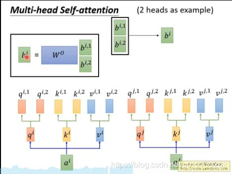
2.3.2 multi-head attention

Multi-head attention 能够使得model关注句子的不同部分,
M u l t i H e a d ( Q , K , V ) = C o n c a t ( h e a d 1 , . . . , h e a d h ) W O where h e a d i = A t t e n t i o n ( Q W i Q , K W i K , V W i V ) \mathrm{MultiHead}(Q, K, V) = \mathrm{Concat}(\mathrm{head_1}, ..., \mathrm{head_h})W^O \\ \text{where}~\mathrm{head_i} = \mathrm{Attention}(QW^Q_i, KW^K_i, VW^V_i) MultiHead(Q,K,V)=Concat(head1,...,headh)WOwhere headi=Attention(QWiQ,KWiK,VWiV)
其中, W i Q ∈ R d model × d k , W i K ∈ R d model × d k , W i V ∈ R d model × d v , W O ∈ R h d v × d model W^Q_i \in \mathbb{R}^{d_{\text{model}} \times d_k}, W^K_i \in \mathbb{R}^{d_{\text{model}} \times d_k}, W^V_i \in \mathbb{R}^{d_{\text{model}} \times d_v}, W^O \in \mathbb{R}^{hd_v \times d_{\text{model}}} WiQ∈Rdmodel×dk,WiK∈Rdmodel×dk,WiV∈Rdmodel×dv,WO∈Rhdv×dmodel。假设head的数目是8,相当于每一个 q i q^i qi中都被分成了8个分支,(下图中是2个分支)。
class MultiHeadedAttention(nn.Module):
    def __init__(self, h, d_model, dropout=0.1):
        "Take in model size and number of heads."
        super(MultiHeadedAttention, self).__init__()
        assert d_model % h == 0
        # We assume d_v always equals d_k
        self.d_k = d_model // h
        self.h = h
        self.linears = clones(nn.Linear(d_model, d_model), 4)
        self.attn = None
        self.dropout = nn.Dropout(p=dropout)

    def forward(self, query, key, value, mask=None):
        "Implements Figure 2"
        if mask is not None:
            # Same mask applied to all h heads.
            mask = mask.unsqueeze(1)
        nbatches = query.size(0)

        # 1) Do all the linear projections in batch from d_model => h x d_k
        # 先对输入值x进行reshape一下,然后交换在维度1,2进行交换
        query, key, value = \
            [l(x).view(nbatches, -1, self.h, self.d_k).transpose(1, 2)
             for l, x in zip(self.linears, (query, key, value))]

        # 2) Apply attention on all the projected vectors in batch.
        x, self.attn = attention(query, key, value, mask=mask,
                                 dropout=self.dropout)

        # 3) "Concat" using a view and apply a final linear.
        x = x.transpose(1, 2).contiguous() \
             .view(nbatches, -1, self.h * self.d_k)
        return self.linears[-1](x)
d_model是个什么玩意?为什么d_k = d_model // h?
To facilitate these residual connections, all sub-layers in the model, as well as the embedding layers, produce outputs of dimension d m o d e l d_{model} dmodel=512.
由此可见, d m o d e l d_{model} dmodel代表的是所有sub-layers输出结果的维度。可以理解为:输出的结果中每个维度都由不同的head组成。
2.4 在模型中使用Attention
在Transformer模型中,在三个不同的地方使用的attention机制:
- encoder-decoder层,queries来自之前的decoder层,memory key和values来自于encoder的输出。这样保证了decoder中每个信息都参与了后面的运算。这一操作的目的是模仿传统attention中的seq2seqmodel。
- 在encoder中包括了self-attention层,self-attention层中的所有key、values、queries都来自于一个place,在这个案例中,这个地方是encode之前的输出值。这样的好处是,每个encoder的信息都包括了之前encoder的信息。
- decoder的self-attention也包括decoder的全部信息,但是需要注意一点的是,我们需要将阻止decoder leftward information flow,来保证auto-regressive property. 实现的方法就是通过masking out方法——即将softmax的输入值设置为 − ∞ -\infty −∞。
2.5 Position-wise Feed-Forward Networks
每个encoder和decoder都包括一个全连接的网络层,变换为:
F F N ( x ) = max ( 0 , x W 1 + b 1 ) W 2 + b 2 \mathrm{FFN}(x)=\max(0, xW_1 + b_1) W_2 + b_2 FFN(x)=max(0,xW1+b1)W2+b2
While the linear transformations are the same across different positions, they use different parameters from layer to layer.
The dimensionality of input and output is d m o d e l = 512 d_{model}=512 dmodel=512 , and the inner-layer has dimensionality d f f = 2048 d_{ff}=2048 dff=2048.
class PositionwiseFeedForward(nn.Module):
    "Implements FFN equation."
    def __init__(self, d_model, d_ff, dropout=0.1):
    	# d_model: attention层的输出结果的维度大小
    	# d_ff: 最终输出结果的维度大小?
        super(PositionwiseFeedForward, self).__init__()
        self.w_1 = nn.Linear(d_model, d_ff)
        self.w_2 = nn.Linear(d_ff, d_model)
        self.dropout = nn.Dropout(dropout)

    def forward(self, x):
        return self.w_2(self.dropout(F.relu(self.w_1(x))))
2.6 Embedding and Softmax
与其他语言模型一样,加上了softmax转化为概率。
class Embeddings(nn.Module):
    def __init__(self, d_model, vocab):
        super(Embeddings, self).__init__()
        self.lut = nn.Embedding(vocab, d_model)
        self.d_model = d_model

    def forward(self, x):
        return self.lut(x) * math.sqrt(self.d_model)
2.7 Position Encoding
由于算法中没有循环以及卷积操作,为了能体现输入数据的时序性,需要在输入时增加序列的相对位置和绝对位置。于是,在编码器和解码器的输入部分,增加位置的编码信息。
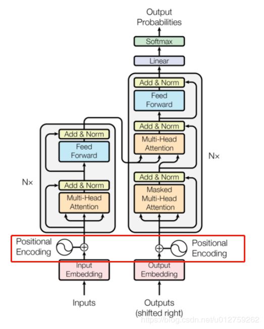
位置编码与输入数据有同样的维度,因此这俩个向量可以相加。
在示例代码中,我们使用 s i n e sine sine 和 c o s i n e cosine cosine函数对位置信息进行编码。编码的范围从 2 π 2\pi 2π到 10000 × 2 π 10000 \times 2\pi 10000×2π。这么做的原因是对于句子中任何一个单词, P E p o s + k PE_{pos+k} PEpos+k都可以表示为 P E p o s PE_{pos} PEpos的线性组合,也就是说,模型能够学习到各个单词的相对位置。
在自然语言处理中,定义一个位置嵌入的概念, 也就是 p o s i t i o n a l e n c o d i n g positional \ encoding positional encoding, 位置嵌入的维度为 [ m a x s e q u e n c e l e n g t h , e m b e d d i n g d i m e n s i o n ] [max \ sequence \ length, \ embedding \ dimension] [max sequence length, embedding dimension], 嵌入的维度同词向量的维度, m a x s e q u e n c e l e n g t h max \ sequence \ length max sequence length属于超参数, 指的是限定的最大单个句长.
注意, 我们一般以字为单位训练transformer模型, 也就是说我们不用分词了, 首先我们要初始化字向量为 [ v o c a b s i z e , e m b e d d i n g d i m e n s i o n ] [vocab \ size, \ embedding \ dimension] [vocab size, embedding dimension], v o c a b s i z e vocab \ size vocab size为总共的字库数量, e m b e d d i n g d i m e n s i o n embedding \ dimension embedding dimension为字向量的维度, 也是每个字的数学表达.
具体公式为:
P E ( p o s , 2 i ) = s i n ( p o s / 1000 0 2 i / d model ) P E ( p o s , 2 i + 1 ) = c o s ( p o s / 1000 0 2 i / d model ) PE_{(pos,2i)} = sin(pos / 10000^{2i/d_{\text{model}}}) \\ PE_{(pos,2i+1)} = cos(pos / 10000^{2i/d_{\text{model}}}) PE(pos,2i)=sin(pos/100002i/dmodel)PE(pos,2i+1)=cos(pos/100002i/dmodel)
上式中 p o s pos pos指的是句中字的位置, 取值范围是 [ 0 , m a x s e q u e n c e l e n g t h ) [0, \ max \ sequence \ length) [0, max sequence length), i i i指的是词向量的维度, 取值范围是 [ 0 , e m b e d d i n g d i m e n s i o n ) [0, \ embedding \ dimension) [0, embedding dimension)。
上面有 s i n sin sin和 c o s cos cos一组公式, 也就是对应着 e m b e d d i n g d i m e n s i o n embedding \ dimension embedding dimension维度的一组奇数和偶数的序号的维度,例如 0 , 1 0, 1 0,1一组, 2 , 3 2, 3 2,3一组, 分别用上面的 s i n sin sin和 c o s cos cos函数做处理, 从而产生不同的周期性变化, 而位置嵌入在 e m b e d d i n g d i m e n s i o n embedding \ dimension embedding dimension维度上随着维度序号增大, 周期变化会越来越慢, 而产生一种包含位置信息的纹理, 就像论文原文中第六页讲的, 位置嵌入函数的周期从 2 π 2 \pi 2π到 10000 ∗ 2 π 10000 * 2 \pi 10000∗2π变化, 而每一个位置在 e m b e d d i n g d i m e n s i o n embedding \ dimension embedding dimension维度上都会得到不同周期的 s i n sin sin和 c o s cos cos函数的取值组合, 从而产生独一的纹理位置信息, 模型从而学到位置之间的依赖关系和自然语言的时序特性.

class PositionalEncoding(nn.Module):
    "Implement the PE function."
    def __init__(self, d_model, dropout, max_len=5000):
        super(PositionalEncoding, self).__init__()
        self.dropout = nn.Dropout(p=dropout)

        # Compute the positional encodings once in log space.
        pe = torch.zeros(max_len, d_model)
        position = torch.arange(0, max_len).unsqueeze(1)
        div_term = torch.exp(torch.arange(0, d_model, 2) *
                             -(math.log(10000.0) / d_model))
        pe[:, 0::2] = torch.sin(position * div_term)
        pe[:, 1::2] = torch.cos(position * div_term)
        pe = pe.unsqueeze(0)
        self.register_buffer('pe', pe)

    def forward(self, x):
        x = x + Variable(self.pe[:, :x.size(1)],
                         requires_grad=False)
        return self.dropout(x)
3 Full Model
def make_model(src_vocab, tgt_vocab, N=6,
               d_model=512, d_ff=2048, h=8, dropout=0.1):
    "Helper: Construct a model from hyperparameters."
    # src_vocab:输入单词的长度
    # tgt_vocab:输出单词的长度
    # d_model: 词向量的长度
    # h: 注意力是几头的
    c = copy.deepcopy
    attn = MultiHeadedAttention(h, d_model)
    ff = PositionwiseFeedForward(d_model, d_ff, dropout)
    position = PositionalEncoding(d_model, dropout)
    model = EncoderDecoder(
        Encoder(
            EncoderLayer(d_model, c(attn), c(ff), dropout),
            N
        ),
        Decoder(
            DecoderLayer(d_model, c(attn), c(attn), c(ff), dropout),
            N
        ),
        nn.Sequential(
            Embeddings(d_model, src_vocab), c(position)
        ),
        nn.Sequential(
            Embeddings(d_model, tgt_vocab), c(position)
        ),
        Generator(d_model, tgt_vocab)
    )

    # This was important from their code.
    # Initialize parameters with Glorot / fan_avg.
    for p in model.parameters():
        if p.dim() > 1:
            nn.init.xavier_uniform(p)
    return model
4. Training
4.1 Batches and Masking
class Batch:
    "Object for holding a batch of data with mask during training."
    def __init__(self, src, trg=None, pad=0):
        self.src = src
        self.src_mask = (src != pad).unsqueeze(-2)
        if trg is not None:
            self.trg = trg[:, :-1]
            self.trg_y = trg[:, 1:]
            self.trg_mask = \
                self.make_std_mask(self.trg, pad)
            self.ntokens = (self.trg_y != pad).data.sum()

    @staticmethod
    def make_std_mask(tgt, pad):
        "Create a mask to hide padding and future words."
        tgt_mask = (tgt != pad).unsqueeze(-2)
        tgt_mask = tgt_mask & Variable(
            subsequent_mask(tgt.size(-1)).type_as(tgt_mask.data))
        return tgt_mask
4.2 training loop
def run_epoch(data_iter, model, loss_compute):
    "Standard Training and Logging Function"
    start = time.time()
    total_tokens = 0
    total_loss = 0
    tokens = 0
    for i, batch in enumerate(data_iter):
        out = model.forward(batch.src, batch.trg,
                            batch.src_mask, batch.trg_mask)
        loss = loss_compute(out, batch.trg_y, batch.ntokens)
        total_loss += loss
        total_tokens += batch.ntokens
        tokens += batch.ntokens
        if i % 50 == 1:
            elapsed = time.time() - start
            print("Epoch Step: %d Loss: %f Tokens per Sec: %f" %
                    (i, loss / batch.ntokens, tokens / elapsed))
            start = time.time()
            tokens = 0
    return total_loss / total_tokens
4.3 Training Data and Batching
作者在英语-德语的数据集上进行了测试,该数据集包括4.5亿个句子。
global max_src_in_batch, max_tgt_in_batch
def batch_size_fn(new, count, sofar):
    "Keep augmenting batch and calculate total number of tokens + padding."
    global max_src_in_batch, max_tgt_in_batch
    if count == 1:
        max_src_in_batch = 0
        max_tgt_in_batch = 0
    max_src_in_batch = max(max_src_in_batch,  len(new.src))
    max_tgt_in_batch = max(max_tgt_in_batch,  len(new.trg) + 2)
    src_elements = count * max_src_in_batch
    tgt_elements = count * max_tgt_in_batch
    return max(src_elements, tgt_elements)
4.4 优化函数
We used the Adam optimizer (cite) with β 1 = 0.9 , β 2 = 0.98 , ϵ = 10 − 9 β_1=0.9, β_2=0.98, \epsilon=10−9 β1=0.9,β2=0.98,ϵ=10−9,学习率根据以下公式进行衰减:
l r a t e = d m o d e l − 0.5 ⋅ min ( s t e p _ n u m − 0.5 , s t e p _ n u m ⋅ w a r m u p _ s t e p s − 1.5 ) l_{rate}=d_{model}^{-0.5} · \min(step\_num^{-0.5}, step\_num · warmup\_steps^{-1.5}) lrate=dmodel−0.5⋅min(step_num−0.5,step_num⋅warmup_steps−1.5)
class NoamOpt:
    "Optim wrapper that implements rate."
    def __init__(self, model_size, factor, warmup, optimizer):
        self.optimizer = optimizer
        self._step = 0
        self.warmup = warmup
        self.factor = factor
        self.model_size = model_size
        self._rate = 0

    def step(self):
        "Update parameters and rate"
        self._step += 1
        rate = self.rate()
        for p in self.optimizer.param_groups:
            p['lr'] = rate
        self._rate = rate
        self.optimizer.step()

    def rate(self, step = None):
        "Implement `lrate` above"
        if step is None:
            step = self._step
        return self.factor * \
            (self.model_size ** (-0.5) *
            min(step ** (-0.5), step * self.warmup ** (-1.5)))

def get_std_opt(model):
    return NoamOpt(model.src_embed[0].d_model, 2, 4000,
            torch.optim.Adam(model.parameters(), lr=0, betas=(0.9, 0.98), eps=1e-9))
4.5 Regularization

在训练过程中,使用的平滑指数为0.1,
class LabelSmoothing(nn.Module):
    "Implement label smoothing."
    def __init__(self, size, padding_idx, smoothing=0.0):
        super(LabelSmoothing, self).__init__()
        self.criterion = nn.KLDivLoss(size_average=False)
        self.padding_idx = padding_idx
        self.confidence = 1.0 - smoothing
        self.smoothing = smoothing
        self.size = size
        self.true_dist = None

    def forward(self, x, target):
        assert x.size(1) == self.size
        true_dist = x.data.clone()
        true_dist.fill_(self.smoothing / (self.size - 2))
        true_dist.scatter_(1, target.data.unsqueeze(1), self.confidence)
        true_dist[:, self.padding_idx] = 0
        mask = torch.nonzero(target.data == self.padding_idx)
        if mask.dim() > 0:
            true_dist.index_fill_(0, mask.squeeze(), 0.0)
        self.true_dist = true_dist
        return self.criterion(x, Variable(true_dist, requires_grad=False))
参考链接
- 标签平滑参考
- pytorch loss function 总结
5. 总结
note:
- 与LSTM不同的是,self-attention通过使用Position Encoding的方式记录时间序列中的信息。
- self-attention中的序列生成方式与lstm不同,而是预先指定生成序列的长度,通过mask的方式替换目标序列中的值,从而达到生成序列的目的。也就是说,target目标维度(batch_size, predict_times, features)中的predict_times代表预测序列的长度。