TensorFlow2利用Auto-MPG数据集实现神经网络回归任务

1. 导入所需的库

import tensorflow as tf
import pandas as pd
import seaborn as sns
import matplotlib.pyplot as plt

for i in [tf, pd, sns]:
    print(i.__name__,": ",i.__version__,sep="")

输出：

tensorflow: 2.2.0
pandas: 0.25.3
seaborn: 0.10.1

2. 下载并导入数据集

Auto MPG数据集主要收集了70年代末到80年代初不同品牌的汽车燃油效率，数据特征有每加仑量程数、气缸数、排量、马力、车重、加速效率、生产年份、生产地、汽车名字等。

官网地址：https://archive.ics.uci.edu/ml/datasets/auto+mpg

2.1 下载数据集

datasetPath = tf.keras.utils.get_file("auto-mpg.data","http://archive.ics.uci.edu/ml/machine-learning-databases/auto-mpg/auto-mpg.data")
datasetPath

输出：

Downloading data from http://archive.ics.uci.edu/ml/machine-learning-databases/auto-mpg/auto-mpg.data
32768/30286 [================================] - 0s 7us/step
Out[3]:
'C:\\Users\\my-pc\\.keras\\datasets\\auto-mpg.data'

2.2 使用Pandas导入数据集

columnNames = ["MPG","Cylinders","Displacement","Horsepower","Weight","Accleration","Model Year","Origin"]
rawDataset = pd.read_csv(datasetPath, names=columnNames, na_values="?",comment="\t",sep=" ",skipinitialspace=True)
dataset = rawDataset.copy()
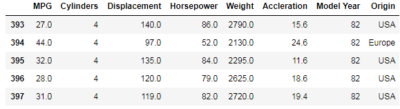
dataset.tail()

输出：

	MPG	Cylinders	Displacement	Horsepower	Weight	Accleration	Model Year	Origin
393	27.0	4	    140.0	        86.0	    2790.0	15.6    	82	        1
394	44.0	4	    97.0	        52.0	    2130.0	24.6    	82        	2
395	32.0	4	    135.0	        84.0	    2295.0	11.6    	82	        1
396	28.0	4	    120.0	        79.0    	2625.0	18.6    	82	        1
397	31.0	4	    119.0	        82.0	    2720.0	19.4    	82	        1

3. 数据清洗

# 统计数据中的NA值
dataset.isna().sum()

输出：

MPG             0
Cylinders       0
Displacement    0
Horsepower      6
Weight          0
Accleration     0
Model Year      0
Origin          0
dtype: int64

可以看到Horsepower列中存在NA值，需要将这些值的样本删除。

dataset = dataset.dropna()
dataset.isna().sum()

输出：

MPG             0
Cylinders       0
Displacement    0
Horsepower      0
Weight          0
Accleration     0
Model Year      0
Origin          0
dtype: int64

dataset["Origin"]

输出：

0      1
1      1
2      1
3      1
4      1
      ..
393    1
394    2
395    1
396    1
397    1
Name: Origin, Length: 392, dtype: int64

Origin列表示汽车的产地，分别用1，2，3存储。但是产地没有大小之分，所以用独热编码更合适。

3.1 方法1

Origin = dataset.pop("Origin")   # 从dataset中删除Origin列
dataset["USA"] = (Origin == 1)*1.0
dataset["Europe"] = (Origin == 2)*1.0
dataset["Japan"] = (Origin == 3)*1.0
dataset.head()

输出：

3.2 方法2

dataset["Origin"] = dataset["Origin"].map({1:"USA",2:"Europe",3:"Japan"})
dataset.tail()

输出：

dataset = pd.get_dummies(dataset, prefix="",prefix_sep="")
dataset.tail()

输出：

3.3 拆分数据集为训练集和测试集

# 按训练集80%，验证集20%的比例拆分
trainDataset = dataset.sample(frac=0.8, random_state=0)
testDataset = dataset.drop(trainDataset.index)
print(trainDataset.shape, testDataset.shape)

输出：

(314, 10) (78, 10)

4. 数据可视化

4.1 绘图展示特征相关性

sns.pairplot(trainDataset[["MPG","Cylinders","Displacement","Weight"]],diag_kind="kde")

输出：

4.2 输出统计指标

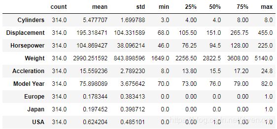
trainStats = trainDataset.describe()
trainStats.pop("MPG")
trainStats = trainStats.transpose()
trainStats

输出：

5. 数据预处理

5.1 拆分训练特征和标签

trainLabels = trainDataset.pop("MPG")
testLabels = testDataset.pop("MPG")
print(trainLabels.shape, testLabels.shape)

输出：

(314,) (78,)

5.2 数据归一化

观察4.2中结果发现，各个特征平均值和标准差相差很大。如果直接拿数据进行建模，使得模型误认为值大的重要程度高，值小的重要程度低。为了避免这种错误的产生，需要对数据进行归一化操作。

常用的归一化有两种方法：

• 1. 标准归一化：(样本值-均值)/标准差，这种归一化的结果为均值为0，方差为1的分布
• 2. 最大最小归一化：(样本值-最小值)/(最大值-最小值)，这种归一化结果为[0,1]的分布

def Norm(x):
    return (x-trainStats["mean"])/trainStats["std"]

normedTrainDataset = Norm(trainDataset)
normedTestDataset = Norm(testDataset)
stat = normedTrainDataset.describe()
stat.transpose()[["mean","std"]]

输出：

6. 模型构建

6.1 构建模型结构

model = tf.keras.Sequential([
    tf.keras.layers.Dense(64,activation="relu",input_shape=[len(trainDataset.keys())]),
    tf.keras.layers.Dense(64,activation="relu"),
    tf.keras.layers.Dense(1)
])
model.summary()

输出：

Model: "sequential_1"
_________________________________________________________________
Layer (type)                 Output Shape              Param #   
=================================================================
dense_3 (Dense)              (None, 64)                640       
_________________________________________________________________
dense_4 (Dense)              (None, 64)                4160      
_________________________________________________________________
dense_5 (Dense)              (None, 1)                 65        
=================================================================
Total params: 4,865
Trainable params: 4,865
Non-trainable params: 0
_________________________________________________________________

6.2 编译模型

optimizer = tf.keras.optimizers.RMSprop(0.001)
model.compile(loss="mse",
             optimizer=optimizer,
             metrics=["mae","mse"])

7. 训练模型

class PrintDot(tf.keras.callbacks.Callback):
    def on_epoch_end(self, epoch, logs):
        if epoch %100 == 0:
            print("")
        print(".",end="")

epochs = 1000
history = model.fit(normedTrainDataset, 
                    trainLabels,
                    epochs=epochs,
                    validation_split=0.2,
                    verbose=0,
                    callbacks=[PrintDot()])

输出：

....................................................................................................
....................................................................................................
....................................................................................................
....................................................................................................
....................................................................................................
....................................................................................................
....................................................................................................
....................................................................................................
....................................................................................................
....................................................................................................

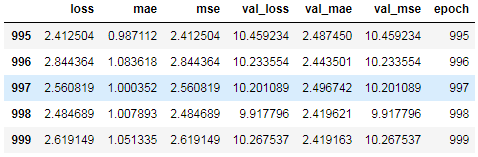
hist = pd.DataFrame(history.history)
hist["epoch"] = history.epoch
hist.tail()

输出：

def plot_history(history):
    hist = pd.DataFrame(history.history)
    hist["epoch"] = history.epoch
    
    plt.figure()
    plt.xlabel("Epoch")
    plt.ylabel("Mean Abs Error [MPG]")
    plt.plot(hist["epoch"],hist["mae"],label="Train Error")
    plt.plot(hist["epoch"],hist["val_mae"],label="Val Error")
    plt.ylim([0,5])
    plt.legend()
    
    plt.figure()
    plt.xlabel('Epoch')
    plt.ylabel('Mean Square Error [$MPG^2$]')
    plt.plot(hist['epoch'], hist['mse'],
           label='Train Error')
    plt.plot(hist['epoch'], hist['val_mse'],
           label = 'Val Error')
    plt.ylim([0,20])
    plt.legend()
    plt.show()

plot_history(history)

输出：

 

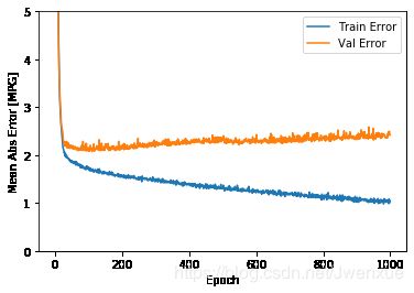
从上图中可以看出，大约训练100之后，训练集上的错误率一直在下降，而验证集上的错误率反而升高了，这表明模型已经过拟合了。此时，我们需要修改模型的训练方式，让模型在验证集错误率不再下降时停止训练，防止过拟合的发生。

model = tf.keras.Sequential([
    tf.keras.layers.Dense(64,activation="relu",input_shape=[len(trainDataset.keys())]),
    tf.keras.layers.Dense(64,activation="relu"),
    tf.keras.layers.Dense(1)
])
model.summary()

optimizer = tf.keras.optimizers.RMSprop(0.001)
model.compile(loss="mse",
             optimizer=optimizer,
             metrics=["mae","mse"])

class PrintDot(tf.keras.callbacks.Callback):
    def on_epoch_end(self, epoch, logs):
        if epoch %100 == 0:
            print("")
        print(".",end="")

epochs = 1000

earlyStop = tf.keras.callbacks.EarlyStopping(monitor="val_loss",patience=10)#当验证集上错误率不再下降时停止训练

history = model.fit(normedTrainDataset, 
                    trainLabels,
                    epochs=epochs,
                    validation_split=0.2,
                    verbose=0,
                    callbacks=[earlyStop,PrintDot()])

plot_history(history)

输出：

Model: "sequential_2"
_________________________________________________________________
Layer (type)                 Output Shape              Param #   
=================================================================
dense_6 (Dense)              (None, 64)                640       
_________________________________________________________________
dense_7 (Dense)              (None, 64)                4160      
_________________________________________________________________
dense_8 (Dense)              (None, 1)                 65        
=================================================================
Total params: 4,865
Trainable params: 4,865
Non-trainable params: 0
_________________________________________________________________

.................................................................

8. 模型评估

利用测试集对训练的模型进行评估

loss, mae, mse = model.evaluate(normedTestDataset, testLabels, verbose=2)
print("Testing set Mean Abs Error: {:5.2f} MPG".format(mae))

输出：

3/3 - 0s - loss: 6.0542 - mae: 1.9105 - mse: 6.0542
Testing set Mean Abs Error:  1.91 MPG

9. 利用模型进行测试

testPredictions = model.predict(normedTestDataset).flatten()

a = plt.axes(aspect="equal")
plt.scatter(testLabels, testPredictions)
plt.xlabel("True Values [MPG]")
plt.ylabel("Predictions [MPG]")
lims = [0,50]
plt.xlim(lims)
plt.ylim(lims)
_ = plt.plot(lims,lims)

输出：

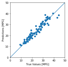
模型预测的结果较好，预测值与真实值几乎相差无几。

error = testPredictions - testLabels
plt.hist(error, bins = 25)
plt.xlabel("Prediction Error [MPG]")
_ = plt.ylabel("Count")

输出：

误差分布并非完全吻合的高斯分布，这可能是由于数据量太小的原因。