2.Iris数据集:感知器模型的简单实战(分类)
一、程序
from sklearn import datasets
import numpy as np
iris=datasets.load_iris()
X=iris.data[:,[2,3]]#2:3才不算3
y=iris.target

a=np.unique(y)#返回类标值

#交叉验证
from sklearn.cross_validation import train_test_split
X_train,X_test,y_train,y_test=train_test_split(X,y,test_size=0.3,random_state=0)

#数据标准化
from sklearn.preprocessing import StandardScaler
sc=StandardScaler()
sc.fit(X_train)#计算得到标准化要的u,方差
X_train_std=sc.transform(X_train)#通过前面计算得到的参数对训练集、测试集分别进行处理
X_test_std=sc.transform(X_test)

#利用训练集进行建模
from sklearn.linear_model import Perceptron
ppn=Perceptron(n_iter=40,eta0=0.1,random_state=0)
ppn.fit(X_train_std,y_train)

#在测试集上运用predict方法进行预测
y_pred=ppn.predict(X_test_std)
print('Misclassified samples:%d' %(y_test!=y_pred).sum())

#计算分类准确率
from sklearn.metrics import accuracy_score
print('Accuracy:%.2f' % accuracy_score(y_test,y_pred))

#绘图
from matplotlib.colors import ListedColormap
import matplotlib.pyplot as plt

def plot_decison_regions(X,y,classifier,test_idx=None,resolution=0.02):

    #设置标记生成器和颜色映射
    markers=('s','x','o','^','v')
    colors=('red','blue','lightgreen','gray','cyan')#一维
    cmap=ListedColormap(colors[:len(np.unique(y))])

    #plot the decision surface
    x1_min,x1_max=X[:,0].min()-1,X[:,0].max()+1
    x2_min,x2_max=X[:,1].min()-1,X[:,0].max()+1
    xx1,xx2=np.meshgrid(np.arange(x1_min,x1_max,resolution),np.arange(x2_min,x2_max,resolution))
    Z=classifier.predict(np.array([xx1.ravel(),xx2.ravel()]).T)
    Z=Z.reshape(xx1.shape)
    plt.contourf(xx1,xx2,Z,alpha=0.4,cmap=cmap)
    plt.xlim(xx1.min(),xx1.max())
    plt.ylim(xx2.min(),xx2.max())

    #plot all samples
    X_test,y_test=X[test_idx,:],y[test_idx]
    for idx,c1 in enumerate(np.unique(y)):
        plt.scatter(x=X[y==c1,0],y=X[y==c1,1],alpha=0.8,c=cmap(idx),marker=markers[idx],label=c1)

    #用于区分哪些是测试集的结果
    if test_idx:
        X_test,y_test=X[test_idx,:],y[test_idx]
        plt.scatter(X_test[:,0],X_test[:,1],c='',alpha=1.0,linewidth=1,marker='o',s=55,label='test set')

#呈现图像
X_combined_std=np.vstack((X_train_std,X_test_std))
y_combined=np.hstack((y_train,y_test))
plot_decison_regions(X=X_combined_std,y=y_combined,classifier=ppn,test_idx=range(105,150))
plt.xlabel('petal length [standardized]')
plt.ylabel('petal length [standardized]')
plt.legend(loc='upper left')
plt.show()
二、展示结果
![]()
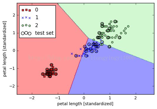
可以看出,45个测试集中有4个分类错误。
附录:
np.meshgrid函数与ravel函数
meshgrid的作用适用于生成网格型数据,可以接受两个一维数组生成两个二维矩阵,对应两个数组中所有的(x,y)对。接下来通过简单的shell交互来演示一下这个功能的使用,并做一下小结。
In [65]: xnums =np.arange(4)

In [66]: ynums =np.arange(5)

In [67]: xnums
Out[67]: array([0,1, 2, 3])

In [68]: ynums
Out[68]: array([0,1, 2, 3, 4])

In [69]: data_list= np.meshgrid(xnums,ynums)

In [70]: data_list
Out[70]:
[array([[0, 1, 2,3],
        [0, 1, 2, 3],
        [0, 1, 2, 3],
        [0, 1, 2, 3],
        [0, 1, 2, 3]]), array([[0, 0, 0, 0],
        [1, 1, 1, 1],
        [2, 2, 2, 2],
        [3, 3, 3, 3],
        [4, 4, 4, 4]])]

In [71]: x,y =data_list
In [72]: x.shape
Out[72]: (5L, 4L)

In [73]: y.shape
Out[73]: (5L, 4L)

In [74]: x
Out[74]:
array([[0, 1, 2,3],
       [0, 1, 2, 3],
       [0, 1, 2, 3],
       [0, 1, 2, 3],
       [0, 1, 2, 3]])

In [75]: y
Out[75]:
array([[0, 0, 0,0],
       [1, 1, 1, 1],
       [2, 2, 2, 2],#如果第一个参数是xarray,维度是xdimesion,第二个参数是yarray,维度是ydimesion。


       [3, 3, 3, 3],# 那么生成的第一个二维数组是以xarray为行,ydimesion行的向量;


       [4, 4, 4, 4]])# 而第二个二维数组是以yarray的转置为列,xdimesion列的向量。
In [13]: x.ravel()
Out[13]: array([0, 1, 2, 3, 0, 1, 2, 3, 0, 1, 2, 3, 0, 1, 2, 3, 0, 1, 2, 3])


In [14]: y.ravel()
Out[14]: array([0, 0, 0, 0, 1, 1, 1, 1, 2, 2, 2, 2, 3, 3, 3, 3, 4, 4, 4, 4])