pytorch 学习笔记 part9 LeNet 模型

LeNet模型

通过Sequential类来实现LeNet模型

#import
import sys
sys.path.append(r"D:\project\letnet学习")
import d2lzh1981 as d2l
import torch
import torch.nn as nn
import torch.optim as optim
import time

#net
class Flatten(torch.nn.Module):  #展平操作
    def forward(self, x):
        return x.view(x.shape[0], -1)

class Reshape(torch.nn.Module): #将图像大小重定型
    def forward(self, x):
        return x.view(-1,1,28,28)      #(B x C x H x W)
    
net = torch.nn.Sequential(     #Lelet                                                  
    Reshape(),
    nn.Conv2d(in_channels=1, out_channels=6, kernel_size=5, padding=2), #b*1*28*28  =>b*6*28*28
    nn.Sigmoid(),                                                       
    nn.AvgPool2d(kernel_size=2, stride=2),                              #b*6*28*28  =>b*6*14*14
    nn.Conv2d(in_channels=6, out_channels=16, kernel_size=5),           #b*6*14*14  =>b*16*10*10
    nn.Sigmoid(),
    nn.AvgPool2d(kernel_size=2, stride=2),                              #b*16*10*10  => b*16*5*5
    Flatten(),                                                          #b*16*5*5   => b*400
    nn.Linear(in_features=16*5*5, out_features=120),
    nn.Sigmoid(),
    nn.Linear(120, 84),
    nn.Sigmoid(),
    nn.Linear(84, 10)
)

构造一个高和宽均为28的单通道数据样本，并逐层进行前向计算来查看每个层的输出形状

#print
X = torch.randn(size=(1,1,28,28), dtype = torch.float32)
for layer in net:
    X = layer(X)
    print(layer.__class__.__name__,'output shape: \t',X.shape)

获取数据和训练模型

# 数据
batch_size = 256
train_iter, test_iter = d2l.load_data_fashion_mnist(
    batch_size=batch_size, root='/home/kesci/input/FashionMNIST2065')
print(len(train_iter))

展示数据的图像

#数据展示
import matplotlib.pyplot as plt
def show_fashion_mnist(images, labels):
    d2l.use_svg_display()
    # 这里的_表示我们忽略（不使用）的变量
    _, figs = plt.subplots(1, len(images), figsize=(12, 12))
    for f, img, lbl in zip(figs, images, labels):
        f.imshow(img.view((28, 28)).numpy())
        f.set_title(lbl)
        f.axes.get_xaxis().set_visible(False)
        f.axes.get_yaxis().set_visible(False)
    plt.show()

for Xdata,ylabel in train_iter:
    break
X, y = [], []
for i in range(10):
    print(Xdata[i].shape,ylabel[i].numpy())
    X.append(Xdata[i]) # 将第i个feature加到X中
    y.append(ylabel[i].numpy()) # 将第i个label加到y中
show_fashion_mnist(X, y)

没有GPU

# This function has been saved in the d2l package for future use
#use GPU
def try_gpu():
    """If GPU is available, return torch.device as cuda:0; else return torch.device as cpu."""
    if torch.cuda.is_available():
        device = torch.device('cuda:0')
    else:
        device = torch.device('cpu')
    return device

device = try_gpu()
device

我们实现evaluate_accuracy函数，该函数用于计算模型net在数据集data_iter上的准确率。

#计算准确率
'''
(1). net.train()
  启用 BatchNormalization 和 Dropout，将BatchNormalization和Dropout置为True
(2). net.eval()
不启用 BatchNormalization 和 Dropout，将BatchNormalization和Dropout置为False
'''

def evaluate_accuracy(data_iter, net,device=torch.device('cpu')):
    """Evaluate accuracy of a model on the given data set.
		data_iter表示测试集，net表示训练的网络，device表示所选用的设备
		acc_sum表示模型预测正确的整数，n表示预测时的总数目
	"""
    acc_sum,n = torch.tensor([0],dtype=torch.float32,device=device),0
    for X,y in data_iter:
        # If device is the GPU, copy the data to the GPU.
        X,y = X.to(device),y.to(device)# 将X,y所表示的tensor变量copy到计算设备中
        net.eval()
        with torch.no_grad():# 该区域不涉及梯度下降和反向传播
            y = y.long()
            acc_sum += torch.sum((torch.argmax(net(X), dim=1) == y))  #[[0.2 ,0.4 ,0.5 ,0.6 ,0.8] ,[ 0.1,0.2 ,0.4 ,0.3 ,0.1]] => [ 4 , 2 ]
            n += y.shape[0]
    return acc_sum.item()/n

定义函数train_ch5，用于训练模型。

#训练函数
def train_ch5(net, train_iter, test_iter,criterion, num_epochs, batch_size, device,lr=None):
    """Train and evaluate a model with CPU or GPU."""
    print('training on', device)
    net.to(device)
    optimizer = optim.SGD(net.parameters(), lr=lr)
    for epoch in range(num_epochs):
        train_l_sum = torch.tensor([0.0],dtype=torch.float32,device=device)
        train_acc_sum = torch.tensor([0.0],dtype=torch.float32,device=device)
        n, start = 0, time.time()
        for X, y in train_iter:
            net.train()
            
            optimizer.zero_grad()
            X,y = X.to(device),y.to(device) 
            y_hat = net(X)
            loss = criterion(y_hat, y)
            loss.backward()
            optimizer.step()
            
            with torch.no_grad():
                y = y.long()
                train_l_sum += loss.float()
                train_acc_sum += (torch.sum((torch.argmax(y_hat, dim=1) == y))).float()
                n += y.shape[0]
        test_acc = evaluate_accuracy(test_iter, net,device)
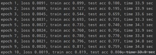
        print('epoch %d, loss %.4f, train acc %.3f, test acc %.3f, '
              'time %.1f sec'
              % (epoch + 1, train_l_sum/n, train_acc_sum/n, test_acc,
                 time.time() - start))

# 训练
lr, num_epochs = 0.9, 10

def init_weights(m):
    if type(m) == nn.Linear or type(m) == nn.Conv2d:
        torch.nn.init.xavier_uniform_(m.weight)

net.apply(init_weights)
net = net.to(device)

criterion = nn.CrossEntropyLoss()   #交叉熵描述了两个概率分布之间的距离，交叉熵越小说明两者之间越接近
train_ch5(net, train_iter, test_iter, criterion,num_epochs, batch_size,device, lr)

# test
for testdata,testlabe in test_iter:
    testdata,testlabe = testdata.to(device),testlabe.to(device)
    break
print(testdata.shape,testlabe.shape)
net.eval()
y_pre = net(testdata)
print(torch.argmax(y_pre,dim=1)[:10])
print(testlabe[:10])