吴恩达Coursera深度学习课程 deeplearning.ai (1-2) 神经网络基础--编程作业
可执行源码:https://download.csdn.net/download/haoyutiangang/10369625
Part 1: Python 基础工具包 Numpy
1 用numpy实现基本方法
1.1 sigmoid 方法 与 np.exp()
利用 np.exp() 方法实现sigmoid方法
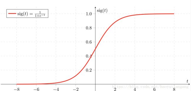
s i g m o i d ( t ) = 1 1 + e − t − − − − − − − − − − − − − − − − − − − − − − − − − − − − s = 1 1 + e − t s ′ = s ( 1 − s ) sigmoid(t) = \frac{1}{1+e^{-t}} \\ ---------------------------- \\ s = \frac{1}{1+e^{-t}} \\ s' = s(1-s) sigmoid(t)=1+e−t1−−−−−−−−−−−−−−−−−−−−−−−−−−−−s=1+e−t1s′=s(1−s)
math.exp(x) : x为一个值
import math
import numpy as np

def basic_sigmoid(x):
    s = 1.0 / (1 + 1/ math.exp(x))
    return s
np.exp(X) : X 为一个向量或矩阵
import numpy as np

def sigmoid(x):
    s = 1.0 / (1 + 1 / np.exp(x))
    return s
补充:声明数组和向量
定义数组:x = np.array([1, 2, 3])
定义向量:x = [1, 2, 3]
1.2 sigmoid 函数的导数
s i g m o i d _ d e r i v a t i v e ( x ) = f ′ ( x ) = f ( x ) ( 1 − f ( x ) ) sigmoid\_derivative(x) = f'(x) = f(x)(1-f(x)) sigmoid_derivative(x)=f′(x)=f(x)(1−f(x))
KaTeX parse error: No such environment: align at position 8: \begin{̲a̲l̲i̲g̲n̲}̲ sigmoid'(t) &=…
def sigmoid_derivative(x):
    s = 1.0 / (1 + 1 / np.exp(x))
    ds = s * (1 - s)
    return ds
1.3 Reshape 数组
- 获取向量或矩阵的维度:X.shape()
- 构造其它维度的向量或矩阵:X.reshape()
Reshape X from 3D array to 1D vector
v = image.reshape((image.shape[0] * image.shape[1] * image.shape[2], 1))
参数中的运算符 * 为拼接只用
def image2vector(image):
    v = image.reshape((image.shape[0] * image.shape[1] * image.shape[2], 1))
    return v
1.4 标准化行
- 矩阵的行标准化:行向量除以行的大小 x/‖x‖
- ‖x‖=np.linalg.norm(x, axis=1, keepdims=True)
- x_normalized = x/‖x‖
def normalizeRows(x):
    x_norm = np.linalg.norm(x, axis=1, keepdims = True)
    x = x / x_norm
    return x
1.5 广播和softmax方法
- 矩阵的广播很重要
softmax function
s o f t m a x ( x ) = e v i ∑ i = 1 n e v i softmax(x) = \frac{e^{v^i}}{\sum_{i=1}^{n}e^{v^i}} softmax(x)=∑i=1nevievi

def softmax(x):
    x_exp = np.exp(x) # (n,m)
    x_sum = np.sum(x_exp, axis = 1, keepdims = True) # (n,1)
    s = x_exp / x_sum  # (n,m) 广播的作用
2 向量化
- np.dot() : 计算内积
- 1维数组,计算内积
- 2维数组,矩阵相乘(推荐 * 或 multiply)
- np.outer() : 计算外积
- 两个等长一维数组:看成向量相乘得矩阵
- * : 分类应用
- 数组:对应相乘
- 矩阵:矩阵相乘
- np.multiply():
- 对应相乘
2.1 实现L1 或 L2 损失函数
L1
- 绝对值: np.abs(x)
L 1 ( y h , y ) = ∑ i = 0 m ∣ y ( i ) − y h ( i ) ∣ L_1(y_h, y) = \sum_{i=0}^{m}|y^{(i)}-y_h^{(i)}| L1(yh,y)=i=0∑m∣y(i)−yh(i)∣
def L1(yhat, y):
    loss = np.sum(np.abs(y - yhat))
    return loss
L2
L 2 ( y h , y ) = ∑ i = 0 m ( y ( i ) − y h ( i ) ) 2 L_2(y_h, y) = \sum_{i=0}^{m}(y^{(i)}-y_h^{(i)})^2 L2(yh,y)=i=0∑m(y(i)−yh(i))2
def L2(yhat, y):
    #loss = np.sum(np.power((y - yhat), 2))
    loss = np.dot(y-yhat,y-yhat)
    return loss
补充
np.sum(X) : 求和
np.dot(1Darray,1Darray) : 内积(也就是对应相乘再加和)
np.multiply(X,Y) : 对应相乘
np.maximum(X) : 求最大值
Part 2: 神经网络倾向的逻辑回归
1 需要导入的包
- numpy: 科学运算
- h5py: 与H5格式文件的交互
- matplotlib: 画图
- PIL and scipy: 测试模型用自己的图
import numpy as np
import matplotlib.pyplot as plt
import h5py
import scipy
from PIL import Image
from scipy import ndimage
from lr_utils import load_dataset

% matplotlib inline
2 浏览数据集
- dataset (“data.h5”)
- shape (num_px, num_px, 3) 猫的图片
- train_set_x_orig, train_set_y, test_set_x_orig, test_set_y 猫的图片集合(set_num, num_px, num_px, 3)
2.1 加载数据集
# Loading the data (cat/non-cat)
train_set_x_orig, train_set_y, test_set_x_orig, test_set_y, classes = load_dataset()
其中 laod_dataset
import numpy as np
import h5py
def load_dataset():
    train_dataset = h5py.File('datasets/train_catvnoncat.h5', "r")
    train_set_x_orig = np.array(train_dataset["train_set_x"][:]) # your train set features
    train_set_y_orig = np.array(train_dataset["train_set_y"][:]) # your train set labels

    test_dataset = h5py.File('datasets/test_catvnoncat.h5', "r")
    test_set_x_orig = np.array(test_dataset["test_set_x"][:]) # your test set features
    test_set_y_orig = np.array(test_dataset["test_set_y"][:]) # your test set labels

    classes = np.array(test_dataset["list_classes"][:]) # the list of classes

    train_set_y_orig = train_set_y_orig.reshape((1, train_set_y_orig.shape[0]))
    test_set_y_orig = test_set_y_orig.reshape((1, test_set_y_orig.shape[0]))

    return train_set_x_orig, train_set_y_orig, test_set_x_orig, test_set_y_orig, classes
2.2 浏览图片
补充
- X[:,index]是numpy中数组的一种写法,表示对一个二维数组,取每一行的第index的值组成一个新的数组,也即矩阵中的第index列
- np.squeeze(array) 删除并返回数组的第一维度
- array.shape[index] 返回第index维度的长度(相当于矩阵的先行后列)
# Example of a picture
index = 25
plt.imshow(train_set_x_orig[index])
print ("y = " + str(train_set_y[:, index]) + ", it's a '" + classes[np.squeeze(train_set_y[:, index])].decode("utf-8") +  "' picture.")

# y = [1], it's a 'cat' picture.
2.3 数据维度
### START CODE HERE ### (≈ 3 lines of code)
m_train = train_set_x_orig.shape[0]  // 第一维
m_test = test_set_x_orig.shape[0]   // 第一维
num_px = train_set_x_orig.shape[1]  // 第二维
### END CODE HERE ###

print ("Number of training examples: m_train = " + str(m_train))
print ("Number of testing examples: m_test = " + str(m_test))
print ("Height/Width of each image: num_px = " + str(num_px))
print ("Each image is of size: (" + str(num_px) + ", " + str(num_px) + ", 3)")
print ("train_set_x shape: " + str(train_set_x_orig.shape))
print ("train_set_y shape: " + str(train_set_y.shape))
print ("test_set_x shape: " + str(test_set_x_orig.shape))
print ("test_set_y shape: " + str(test_set_y.shape))

# Number of training examples: m_train = 209
# Number of testing examples: m_test = 50
# Height/Width of each image: num_px = 64
# Each image is of size: (64, 64, 3)
# train_set_x shape: (209, 64, 64, 3)
# train_set_y shape: (1, 209)
# test_set_x shape: (50, 64, 64, 3)
# test_set_y shape: (1, 50)
2.4 数据整理
补充
# reshape (num_px, num_px, 3)  to (num_px ∗ num_px ∗ 3, 1)
X_flatten = X.reshape(1, -1).T // 自动推测二维,形成行向量,转置形成列向量

# reshape(a,b,c,d) to (b∗c∗d, a)
X_flatten = X.reshape(X.shape[0], -1).T
整理
train_set_x_flatten = train_set_x_orig.reshape(m_train, -1).T
test_set_x_flatten = test_set_x_orig.reshape(m_test, -1).T

print ("train_set_x_flatten shape: " + str(train_set_x_flatten.shape))
print ("train_set_y shape: " + str(train_set_y.shape))
print ("test_set_x_flatten shape: " + str(test_set_x_flatten.shape))
print ("test_set_y shape: " + str(test_set_y.shape))
print ("sanity check after reshaping: " + str(train_set_x_flatten[0:5,0]))

# train_set_x_flatten shape: (12288, 209)
# train_set_y shape: (1, 209)
# test_set_x_flatten shape: (12288, 50)
# test_set_y shape: (1, 50)
# sanity check after reshaping: [17 31 56 22 33]
2.5 中心化和标准化
一般除以中心值,对于图像来说,这里除以最大值255即可
train_set_x = train_set_x_flatten/255.
test_set_x = test_set_x_flatten/255.
2.6 总结
常见步骤
- 计算维度:m_train, m_test, num_px, …
- 整理数据集 Reshape Dataset
- 中心化和标准化
3 学习算法的一般架构

步骤
- 初始化模型参数
- 通过学习来修改模型参数使损失函数取值最小化
- 利用学习的参数在测试集上做测试
- 分析结果并总结
4 构建算法的各个部分
神经网络的主要步骤:
- 定义模型结构(例如输入特征的个数)
- 初始化模型参数
- 循环
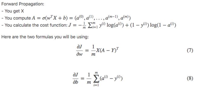
- 计算损失函数(前向传播:forward propagation)
- 计算梯度(反向传播:backward propagation)
- 更新参数(梯度下降:gradient descent)
通常集成1-3到一个model()方法里
4.1 激活函数
s i g m o i d ( w T x + b ) = 1 1 + e − w T x + b sigmoid(w^Tx+b) = \frac{1}{1+e^{-{w^Tx+b}}} sigmoid(wTx+b)=1+e−wTx+b1
def sigmoid(z):
    s = 1.0/(1+np.exp(-z))
    return s
4.2 初始化参数
def initialize_with_zeros(dim):
    w = np.zeros((dim, 1)) // 一维列向量
    b = 0
    assert(w.shape == (dim, 1))
    assert(isinstance(b, float) or isinstance(b, int))
4.3 前向传播和反向传播
# GRADED FUNCTION: propagate

def propagate(w, b, X, Y):
    """
    Implement the cost function and its gradient for the propagation explained above

    Arguments:
    w -- weights, a numpy array of size (num_px * num_px * 3, 1)
    b -- bias, a scalar
    X -- data of size (num_px * num_px * 3, number of examples)
    Y -- true "label" vector (containing 0 if non-cat, 1 if cat) of size (1, number of examples)

    Return:
    cost -- negative log-likelihood cost for logistic regression
    dw -- gradient of the loss with respect to w, thus same shape as w
    db -- gradient of the loss with respect to b, thus same shape as b

    Tips:
    - Write your code step by step for the propagation. np.log(), np.dot()
    """

    m = X.shape[1]

    # FORWARD PROPAGATION (FROM X TO COST)
    ### START CODE HERE ### (≈ 2 lines of code)
    A = sigmoid(np.dot(w.T, X)+b)                                    # compute activation
    cost = -(1.0/m)*np.sum(Y*np.log(A)+(1-Y)*np.log(1-A))                                 # compute cost
    ### END CODE HERE ###

    # BACKWARD PROPAGATION (TO FIND GRAD)
    ### START CODE HERE ### (≈ 2 lines of code)
    dw = (1.0/m)*np.dot(X,(A-Y).T)
    db = (1.0/m)*np.sum(A-Y)
    ### END CODE HERE ###

    assert(dw.shape == w.shape)
    assert(db.dtype == float)
    cost = np.squeeze(cost)
    assert(cost.shape == ())

    grads = {"dw": dw,
             "db": db}

    return grads, cost
4.4 参数调优
# GRADED FUNCTION: optimize

def optimize(w, b, X, Y, num_iterations, learning_rate, print_cost = False):
    """
    This function optimizes w and b by running a gradient descent algorithm

    Arguments:
    w -- weights, a numpy array of size (num_px * num_px * 3, 1)
    b -- bias, a scalar
    X -- data of shape (num_px * num_px * 3, number of examples)
    Y -- true "label" vector (containing 0 if non-cat, 1 if cat), of shape (1, number of examples)
    num_iterations -- number of iterations of the optimization loop
    learning_rate -- learning rate of the gradient descent update rule
    print_cost -- True to print the loss every 100 steps

    Returns:
    params -- dictionary containing the weights w and bias b
    grads -- dictionary containing the gradients of the weights and bias with respect to the cost function
    costs -- list of all the costs computed during the optimization, this will be used to plot the learning curve.

    Tips:
    You basically need to write down two steps and iterate through them:
        1) Calculate the cost and the gradient for the current parameters. Use propagate().
        2) Update the parameters using gradient descent rule for w and b.
    """

    costs = []

    for i in range(num_iterations):


        # Cost and gradient calculation (≈ 1-4 lines of code)
        ### START CODE HERE ###
        grads, cost = propagate(w, b, X, Y)
        ### END CODE HERE ###

        # Retrieve derivatives from grads
        dw = grads["dw"]
        db = grads["db"]

        # update rule (≈ 2 lines of code)
        ### START CODE HERE ###
        w = w - learning_rate*dw
        b = b - learning_rate*db
        ### END CODE HERE ###

        # Record the costs
        if i % 100 == 0:
            costs.append(cost)

        # Print the cost every 100 training examples
        if print_cost and i % 100 == 0:
            print ("Cost after iteration %i: %f" %(i, cost))

    params = {"w": w,
              "b": b}

    grads = {"dw": dw,
             "db": db}

    return params, grads, costs
4.5 预测
# GRADED FUNCTION: predict

def predict(w, b, X):
    '''
    Predict whether the label is 0 or 1 using learned logistic regression parameters (w, b)

    Arguments:
    w -- weights, a numpy array of size (num_px * num_px * 3, 1)
    b -- bias, a scalar
    X -- data of size (num_px * num_px * 3, number of examples)

    Returns:
    Y_prediction -- a numpy array (vector) containing all predictions (0/1) for the examples in X
    '''

    m = X.shape[1]
    Y_prediction = np.zeros((1,m))
    w = w.reshape(X.shape[0], 1)

    # Compute vector "A" predicting the probabilities of a cat being present in the picture
    ### START CODE HERE ### (≈ 1 line of code)
    A = sigmoid(np.dot(w.T, X) + b)
    ### END CODE HERE ###

    for i in range(A.shape[1]):

        # Convert probabilities A[0,i] to actual predictions p[0,i]
        ### START CODE HERE ### (≈ 4 lines of code)
        if A[0,i] > 0.5:
            Y_prediction[0,i] = 1
        else:
            Y_prediction[0,i] = 0
        ### END CODE HERE ###

    assert(Y_prediction.shape == (1, m))

    return Y_prediction
5 整合代码到 model
5.1 整合代码
# GRADED FUNCTION: model

def model(X_train, Y_train, X_test, Y_test, num_iterations = 2000, learning_rate = 0.5, print_cost = False):
    """
    Builds the logistic regression model by calling the function you've implemented previously

    Arguments:
    X_train -- training set represented by a numpy array of shape (num_px * num_px * 3, m_train)
    Y_train -- training labels represented by a numpy array (vector) of shape (1, m_train)
    X_test -- test set represented by a numpy array of shape (num_px * num_px * 3, m_test)
    Y_test -- test labels represented by a numpy array (vector) of shape (1, m_test)
    num_iterations -- hyperparameter representing the number of iterations to optimize the parameters
    learning_rate -- hyperparameter representing the learning rate used in the update rule of optimize()
    print_cost -- Set to true to print the cost every 100 iterations

    Returns:
    d -- dictionary containing information about the model.
    """

    ### START CODE HERE ###

    # initialize parameters with zeros (≈ 1 line of code)
    w, b = initialize_with_zeros(X_train.shape[0])

    # Gradient descent (≈ 1 line of code)
    parameters, grads, costs = optimize(w, b, X_train, Y_train, num_iterations, learning_rate, print_cost)

    # Retrieve parameters w and b from dictionary "parameters"
    w = parameters["w"]
    b = parameters["b"]

    # Predict test/train set examples (≈ 2 lines of code)
    Y_prediction_test = predict(w, b, X_test)
    Y_prediction_train = predict(w, b, X_train)

    ### END CODE HERE ###

    # Print train/test Errors
    print("train accuracy: {} %".format(100 - np.mean(np.abs(Y_prediction_train - Y_train)) * 100))
    print("test accuracy: {} %".format(100 - np.mean(np.abs(Y_prediction_test - Y_test)) * 100))


    d = {"costs": costs,
         "Y_prediction_test": Y_prediction_test,
         "Y_prediction_train" : Y_prediction_train,
         "w" : w,
         "b" : b,
         "learning_rate" : learning_rate,
         "num_iterations": num_iterations}

    return d
5.2 验证
# Example of a picture that was wrongly classified.
index = 1
plt.imshow(test_set_x[:,index].reshape((num_px, num_px, 3)))
print ("y = " + str(test_set_y[0,index]) + ", you predicted that it is a \"" + classes[d["Y_prediction_test"][0,index]].decode("utf-8") +  "\" picture.")
5.3 梯度下降图
# Example of a picture that was wrongly classified.
index = 1
plt.imshow(test_set_x[:,index].reshape((num_px, num_px, 3)))
print ("y = " + str(test_set_y[0,index]) + ", you predicted that it is a \"" + classes[d["Y_prediction_test"][0,index]].decode("utf-8") +  "\" picture.")
6 继续分析
learning_rates = [0.01, 0.001, 0.0001]
models = {}
for i in learning_rates:
    print ("learning rate is: " + str(i))
    models[str(i)] = model(train_set_x, train_set_y, test_set_x, test_set_y, num_iterations = 1500, learning_rate = i, print_cost = False)
    print ('\n' + "-------------------------------------------------------" + '\n')

for i in learning_rates:
    plt.plot(np.squeeze(models[str(i)]["costs"]), label= str(models[str(i)]["learning_rate"]))

plt.ylabel('cost')
plt.xlabel('iterations')

legend = plt.legend(loc='upper center', shadow=True)
frame = legend.get_frame()
frame.set_facecolor('0.90')
plt.show()
7 试验你自己的图片
## START CODE HERE ## (PUT YOUR IMAGE NAME)
my_image = "isacatornot.jpg"   # change this to the name of your image file
## END CODE HERE ##

# We preprocess the image to fit your algorithm.
fname = "images/" + my_image
image = np.array(ndimage.imread(fname, flatten=False))
my_image = scipy.misc.imresize(image, size=(num_px,num_px)).reshape((1, num_px*num_px*3)).T
my_predicted_image = predict(d["w"], d["b"], my_image)

plt.imshow(image)
print("y = " + str(np.squeeze(my_predicted_image)) + ", your algorithm predicts a \"" + classes[int(np.squeeze(my_predicted_image)),].decode("utf-8") +  "\" picture.")