计算机图形学：光线追踪

1.Ray Tracing Algorithm

IntersectColor( vBeginPoint, vDirection)
{
    Determine IntersectPoint;
    Color = ambient color;
    for each light
        Color += local shading term; 
    if(surface is reflective)
        color += reflect Coefficient * IntersectColor(IntersecPoint, ReflectRay);
    else if ( surface is refractive) 
        color += refract Coefficient * IntersectColor(IntersecPoint, Refract Ray);
    return color; 
}

行列式(determinant)

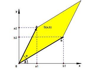
行列式就是行列式中的行或列向量所构成的超平行多面体的有向面积或有向体积

$$\mathbf{d}\mathbf{e}\mathbf{t}(\mathbf{M})=\left|\begin{array}{ccc}{M}_{11}& M_{12}& M_{13}\\ M_{21}& M_{22}& M_{23}\\ M_{31}& M_{32}& M_{33}\end{array}\right|$$

• 二阶行列式的几何意义就是由行列式的向量所张成的平行四边形的面积
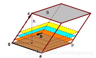
• 一个3×3阶的行列式是其行向量或列向量所张成的平行六面体的有向体积

代数余子式${\mathbf{C}}_{\mathbf{i}\mathbf{j}}(\mathbf{M})=(-1{)}^{\mathbf{i}+\mathbf{j}}\mathbf{d}\mathbf{e}\mathbf{t}({\mathbf{M}}^{\{\mathbf{i},\mathbf{j}\}})$,其中${\mathbf{M}}^{\{\mathbf{i},\mathbf{j}\}}$是去除i行和j列后的矩阵

矩阵M的行列式等于任意一行或者一列元素与其代数余子式乘积的和

$$\begin{gathered} \mathbf{d}\mathbf{e}\mathbf{t}(\mathbf{M})=\sum _{\mathbf{i}=1}^{\mathbf{n}}{\mathbf{M}}_{\mathbf{i}\mathbf{k}}{\mathbf{C}}_{\mathbf{i}\mathbf{k}}(\mathbf{M}) \\ \mathbf{d}\mathbf{e}\mathbf{t}(\mathbf{M})=\sum _{\mathbf{j}=1}^{\mathbf{n}}{\mathbf{M}}_{\mathbf{k}\mathbf{j}}{\mathbf{C}}_{\mathbf{k}\mathbf{j}}(\mathbf{M}) \end{gathered}$$

克莱姆法则（Cramer’s Rule）

一个线性方程组可以用矩阵（M为n*n的方阵）与向量（X，C均长度为n的列向量）的方程来表示：

$$\mathbf{M}\mathbf{X}=\mathbf{C}$$

如果M是一个可逆矩阵，那么方程有解，为

$${\mathbf{X}}_{\mathbf{i}}=\frac{\mathbf{d}\mathbf{e}\mathbf{t}({\mathbf{M}}_{\mathbf{i}})}{\mathbf{d}\mathbf{e}\mathbf{t}(\mathbf{M})}$$

其中${\mathbf{M}}_{\mathbf{i}}$是被列向量C取代了M的第i列的列向量后得到的矩阵。

混合积的运算法则

1.混合积和三维矩阵行列式的关系

其中后一个等号矩阵的转置矩阵的行列式等于这个矩阵的行列式

$$\mathbf{a}\cdot (\mathbf{b}\times \mathbf{c})=\left|\begin{array}{ccc}{a}_1& a_2& a_3\\ b_1& b_2& b_3\\ c_1& c_2& c_3\end{array}\right|=\left|\begin{array}{ccc}{a}_1& b_1& c_1\\ a_2& b_2& c_2\\ a_3& b_3& c_3\end{array}\right|$$

2.混合积的交换律

$$\mathbf{a}\cdot (\mathbf{b}\times \mathbf{c})=\mathbf{b}\cdot (\mathbf{c}\times \mathbf{a})=\mathbf{c}\cdot (\mathbf{a}\times \mathbf{b})$$

2.Ray intersection(光线求交)

2.1 Ray Representation

$$\mathbf{P}(\mathbf{t})={\mathbf{R}}_{\mathbf{o}}+\mathbf{t}\ast {\mathbf{R}}_{\mathbf{d}}$$

2.2 Plane intersection

平面表示:

$$\mathbf{H}(\mathbf{P})=\mathbf{A}\mathbf{x}+\mathbf{B}\mathbf{y}+\mathbf{C}\mathbf{z}+\mathbf{D}=\mathbf{n}\cdot \mathbf{P}+\mathbf{D}=0$$

n为法向量，D为距离原点的偏移

联立方程

$$\begin{gathered} \mathbf{P}(\mathbf{t})={\mathbf{R}}_{\mathbf{o}}+\mathbf{t}\ast {\mathbf{R}}_{\mathbf{d}} \\ \mathbf{n}\cdot \mathbf{P}(\mathbf{t})+\mathbf{D}=0 \\ \mathbf{t}=-\frac{\mathbf{D}+\mathbf{n}\cdot \mathbf{R}\mathbf{o}}{(\mathbf{n}\cdot \mathbf{R}\mathbf{d})} \end{gathered}$$

2.3 Triangle intersection

• 第一步：判断三角形所在的面和线段所在的直线是否平行或者是否是从三角形面的背面进入。如果是就提前退出，否则进入第二步。（使用面的法向量 和 线段的向量 的 点积）

• 第二步：判断线段和三角形所在的面的交点是否在线段上。

• 第三步：判断是否交点在三角形内部。

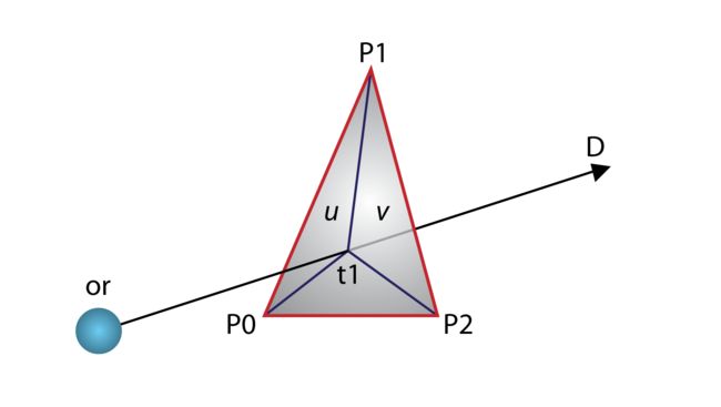
重心坐标系（Barycentric coordinates）:

Barycentric coordinates could be used for texture mapping, normal interpolation, color interpolation, etc.

$$\mathbf{P}=\alpha {\mathbf{P}}_0+\beta {\mathbf{P}}_1+\gamma {\mathbf{P}}_2\alpha +\beta +\gamma =10⩽\alpha ,\beta ,\gamma ⩽1$$

相交检测：

$$\begin{gathered} \mathbf{P}(\mathbf{t})={\mathbf{R}}_{\mathbf{o}}+\mathbf{t}\ast {\mathbf{R}}_{\mathbf{d}}=(1-\beta -\gamma ){\mathbf{P}}_0+\beta {\mathbf{P}}_1+\gamma {\mathbf{P}}_2 \\ ({\mathbf{R}}_{\mathbf{d}},{\mathbf{P}}_0-{\mathbf{P}}_1,{\mathbf{P}}_0-{\mathbf{P}}_2)\left(\begin{array}{c}t\\ \beta \\ \gamma \end{array}\right)={\mathbf{P}}_0-{\mathbf{R}}_{\mathbf{o}} \end{gathered}$$

克莱姆法则:

$$\begin{gathered} {\mathbf{E}}_1={\mathbf{P}}_0-{\mathbf{P}}_1,{\mathbf{E}}_2={\mathbf{P}}_0-{\mathbf{P}}_2,\mathbf{S}={\mathbf{P}}_0-{\mathbf{R}}_{\mathbf{o}} \\ \left(\begin{array}{c}t\\ \beta \\ \gamma \end{array}\right)=\frac{1}{\mathbf{d}\mathbf{e}\mathbf{t}({\mathbf{R}}_{\mathbf{d}},{\mathbf{E}}_1,{\mathbf{E}}_2)}\left(\begin{array}{c}det(S,E_1,E_2)\\ det(R_d,S,E_2)\\ det(R_d,E_1,S)\end{array}\right) \end{gathered}$$

2.4 Polygon intersection

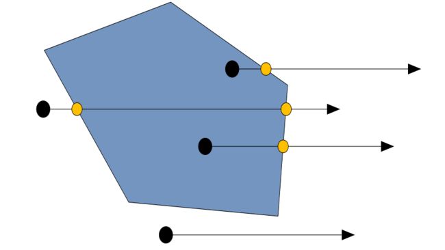
Crossing Test

从点引出一根“射线”，与多边形的任意若干条边相交，累计相交的边的数目，如果是奇数，那么点就在多边形内，否则点就在多边形外。

2.5 Sphere intersection

Algebra Solution:

$$\begin{gathered} (\mathbf{P}-{\mathbf{P}}_{\mathbf{c}})\cdot (\mathbf{P}-{\mathbf{P}}_{\mathbf{c}})={\mathbf{R}}^2 \\ ({\mathbf{R}}_{\mathbf{o}}+\mathbf{t}\ast {\mathbf{R}}_{\mathbf{d}}-{\mathbf{P}}_{\mathbf{c}})\cdot ({\mathbf{R}}_{\mathbf{o}}+\mathbf{t}\ast {\mathbf{R}}_{\mathbf{d}}-{\mathbf{P}}_{\mathbf{c}})={\mathbf{R}}^2 \\ {\mathbf{R}}_{\mathbf{d}}\cdot {\mathbf{R}}_{\mathbf{d}}\ast {\mathbf{t}}^2+2{\mathbf{R}}_{\mathbf{d}}\cdot ({\mathbf{R}}_{\mathbf{o}}-{\mathbf{P}}_{\mathbf{c}})\ast \mathbf{t}+({\mathbf{R}}_{\mathbf{o}}-{\mathbf{P}}_{\mathbf{c}})\cdot ({\mathbf{R}}_{\mathbf{o}}-{\mathbf{P}}_{\mathbf{c}})-{\mathbf{R}}^2=0 \end{gathered}$$

Geometric Method

Is ray origin inside/outside the sphere?

• ${\mathbf{l}}^2>{\mathbf{R}}^2$ Outside the sphere
• ${\mathbf{l}}^2={\mathbf{R}}^2$ On the sphere
• ${\mathbf{l}}^2<{\mathbf{R}}^2$ Inside the sphere

$$\begin{gathered} \mathbf{l}={\mathbf{P}}_{\mathbf{c}}-{\mathbf{R}}_{\mathbf{o}} \\ {\mathbf{t}}_{\mathbf{p}}=\mathbf{l}\cdot {\mathbf{R}}_{\mathbf{d}} \\ \mathbf{D}=\sqrt{{\mathbf{l}}^2-{{\mathbf{t}}_{\mathbf{p}}}^2} \end{gathered}$$

If D>R , no hit

$${{\mathbf{t}}^{\prime }}^2={\mathbf{R}}^2-{\mathbf{D}}^2$$

• If origin outside sphere $\mathbf{t}={\mathbf{t}}_{\mathbf{p}}-{\mathbf{t}}^{\prime }$
• If origin inside sphere $\mathbf{t}={\mathbf{t}}_{\mathbf{p}}+{\mathbf{t}}^{\prime }$

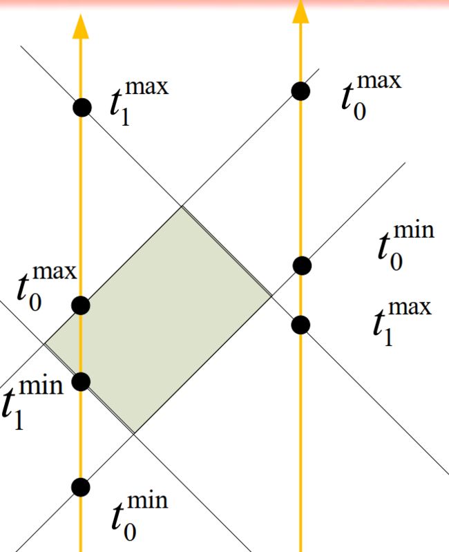
2.6 Box intersection

Foreachslab,intersecting with the ray,there is a minimum t value and maximum t value, these are called ${\mathbf{t}}_{\mathbf{i}}^{\mathbf{m}\mathbf{i}\mathbf{n}}$ and ${\mathbf{t}}_{\mathbf{i}}^{\mathbf{m}\mathbf{a}\mathbf{x}}$ ,(i=0, 1, 2)

The next step is to compute:
$$\begin{gathered} {\mathbf{t}}_{}^{\mathbf{m}\mathbf{i}\mathbf{n}}=\mathbf{m}\mathbf{a}\mathbf{x}({\mathbf{t}}_0^{\mathbf{m}\mathbf{i}\mathbf{n}},{\mathbf{t}}_1^{\mathbf{m}\mathbf{i}\mathbf{n}},{\mathbf{t}}_2^{\mathbf{m}\mathbf{i}\mathbf{n}}) \\ {\mathbf{t}}_{}^{\mathbf{m}\mathbf{a}\mathbf{x}}=\mathbf{m}\mathbf{i}\mathbf{n}({\mathbf{t}}_0^{\mathbf{m}\mathbf{a}\mathbf{x}},{\mathbf{t}}_1^{\mathbf{m}\mathbf{a}\mathbf{x}},{\mathbf{t}}_2^{\mathbf{m}\mathbf{a}\mathbf{x}}) \end{gathered}$$

• if${\mathbf{t}}_{}^{\mathbf{m}\mathbf{i}\mathbf{n}}<{\mathbf{t}}_{}^{\mathbf{m}\mathbf{a}\mathbf{x}}$ ,then the ray intersects the box
  ${\mathbf{t}}_{}^{\mathbf{m}\mathbf{i}\mathbf{n}}$ is the enter-point, ${\mathbf{t}}_{}^{\mathbf{m}\mathbf{a}\mathbf{x}}$ is the exit point
• Otherwise, no intersections