Spherical Harmonic Lighting: The Gritty Details

http://silviojemma.com/public/papers/lighting/spherical-harmonic-lighting.pdf
https://huailiang.github.io/blog/2019/harmonics/
https://www.gdcvault.com/play/1015312/Light-Probe-Interpolation-Using-Tetrahedral
http://silviojemma.com/public/papers/lighting/spherical-harmonic-lighting.pdf
https://sites.fas.harvard.edu/~cs278/papers/prt.pdf
https://github.com/TianYiJT/SphericalHarmonicLighting 有源码

Spherical Harmonic lighting (SH lighting) is a technique for calculating the lighting on 3D models from area light sources that allows us to capture, relight and display global illumination style images in real time. It was introduced in a paper at Siggraph 2002 by Sloan, Kautz and Snyder https://sites.fas.harvard.edu/~cs278/papers/prt.pdf as a technique for ultra realistic lighting of models. Looking a little closer at it’s derivation we can show that it is in fact a toolbox of interrelated 相互关联的 techniques that the games community can use to good effect.

The results are compelling and the code to compute them is actually straightforward to write, but the paper that introduces it assumes a lot of background knowledge from the first time reader. This paper is an attempt to provide this background, add some insights into the “why” questions, and hopefully give you all you need to add SH lighting to your game.

If you have spent any time coding a 3D engine you should be familiar with the common lighting models, and concepts like specular highlights, diffuse colors and ambient lights should be second nature to you. The simplest lighting model that you probably use is the diffuse surface reflection model sometimes known as “dot product lighting”. For each light source the intensity (often expressed as an RGB colour) is multiplied by the scalar dot product between the unit surface normal N and the unit vector towards the light source L. This value is then multiplied by the surface colour giving the final reflected result:

One way of looking at this code fragment is to say that it first calculates the total amount of incoming light from all directions, then scales it by the cosine of the angle between N and L and multiplies the result by the surface reflection function (which for a diffuse surface is just a constant colour for all directions). This is a simplification of the rendering equation, a formulation of the problem of producing images in computer graphics that is based only on physics. It is the gold standard by which all realistic computer graphics lighting must be measured. The problem with the rendering equation is that it is difficult to compute, and definitely not a real-time friendly operation. It is an integral over a hemisphere of directions where L, the light intensity function we are looking to calculate, appears on both sides of the equation:

To anyone used to writing raytracers the only difficult concept is the use of differential angles to represent rays and solving the actual integral itself, but the background is quite simple. I urge you to learn more about global illumination solutions as for this tutorial all I can give you is a taster. Imagine that time is stationary 静止的. Picture a volume of space filled with photons – each cube of space can be said to have a constant photon density. Picture this field of photons in linear motion. At the very heart of rendering, we need to find out how many photons collide with a stationary surface for each unit of time, a value called flux which measured in joules/second or watts.

To calculate the flux, note that all the photons that will hit the surface within a unit of time t lie within the volume swept behind the surface in the direction of flow – as the angle gets shallower 浅, less photons hit the surface per unit of time because the swept volume is smaller. The relationship turns out to be proportional to the cosine of the angle between the surface normal and the direction of flow. As the lengths of the sides of this patch tend towards zero, we get the differential area of the patch. Dividing the flux by the differential area, we get a value called the irradiance, measured in watts/meter2. That’s the idea for one small patch and one direction of incoming light, but the relationship also holds when we consider all directions visible from a surface, as shown in Figure 2. As the angle gets shallower the projected area approaches zero. This is the reason behind the cosine (or dot product) in the diffuse shading equation.

That was just a quick taste of the background to the rendering equation, but I hope you can see that by looking more carefully at the derivation of our shading models and paying attention to the details we should be able calculate extremely realistic images based on purely physical principles. The only question left is how can we do this in real time? As a games programmer you may look at the rendering equation and throw your hands up in horror 被吓着了. An integral inside the inner loop of a shader? And how do we “integrate over a hemisphere”? How does this relate to any kind of hardware operations we have available? The rest of this document aims to take these abstract definitions and propose methods for calculating global illumination solutions and displaying them in a game friendly manner.

Monte Carlo Integration
We have a function to integrate, the function describing incoming light intensity, but we have no idea what that function looks like so there is no way we can calculate a result symbolically 象征性的. The key to unlocking the puzzle is called Monte Carlo Integration, and it’s all related to probability. First, some background in probability theory. A random variable is a value that lies within a specific domain with some distribution of values. For example, rolling a single 6-sided dice will return a discrete value from the set fi = {1,2,3,4,5,6} where each value has equal probability of occurring of pi = 1/6. The cumulative distribution function P(x) is just a function that tells us the probability that when we roll a die, we will roll a value less than x.

For example the probability that rolling a die will return a value less than 4 is P(4) = 2/3. If a variable has equal probability of taking any value within it’s range it is known as a uniform random variable 均匀随机变量. Rolling a die returns a discrete value for each turn – there
are no fractional values it could return - but random variables can also have a continuous range, for example picking a random number within the range [3,7]. One continuous variable that turns up time and time again is the uniform random variable that produces values in the range [0,1) (i.e. including 0, excluding 1), and it is so useful for generating samples from other distributions it is sometimes called the canonical random variable and we will denoted it with the symbol ξ.

The function we are most likely to be working with is the probability density function (PDF) which tells us the relative probability that a variable will take on a specific value, and is defined as the derivative of the cumulative distribution function. Random variables are said to be distributed according to a particular PDF, and this is denoted by writing f(x) ~ p(x). PDFs have positive or zero values for every valid number in the range and the function must integrate to 1.

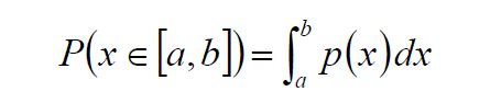
The probability that a variable x will take a value in the range [a,b] is just the integral between a and b of the PDF.

Every function using a random variable has an average value, the mean value, that it will tend to return most often if you take many, many samples. This is termed the expected value of the function, written E[f(x)], which is calculated as:

For example, let’s find the expected or mean value for f(x)=2-x over the range [0…2]. In order for the function to integrate to 1 over the range, we need to set p(x)=1/2. The integral gives us:

Another way of calculating the expected value of a function is to take the mean of a large number of random samples from the function, which can be shown to converge towards the correct answer as the number of samples approaches infinity (called the Law of Large Numbers):

We can combine these two results in one of the sneakiest 卑鄙的 tricks in the whole of Engineering Mathematics to give us an estimate of the integral of a function

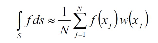
We just take lots and lots of point samples of the function f(x), scale each one by the PDF, sum the result and divide by the number of samples at the end. Intuitively you can see that samples with a higher probability of occurring are given less weight in the final answer. The other intuition from this equation is that distributions that are similar to the function being integrated have less variance in their answers, ending up with only a single sample being needed when p(x) = f(x). Another way of writing the Monte Carlo Estimator is to multiply each sample by a weighting function w(x) = 1/p(x) instead of dividing by the probability, leading us to the final form of the Monte Carlo Estimator:

If we can guarantee that p(x) is a uniform distribution over the space we want to sample then we can just take point samples of our function, sum them, divide by the number of samples times w(x) and we have calculated an approximation to the integral of our function saving many multiplies. We know from the rendering equation that we want to integrate over the surface of a sphere, so all we need to do is generate evenly distributed points (more technically called unbiased random samples) over the surface of a sphere. Taking a pair of independent canonical random numbers ξx and ξy we can map this “square” of random values into spherical coordinates using the transform:

The probability that we will sample any point on the surface of this unit sphere is the same for all samples, meaning that our
weighting function is just the constant value 1/the surface area of a sphere, giving us a weighting function of w(x) = 4π. The
resulting distribution of points is shown below.

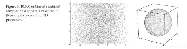
An additional tool, to lower the variance 方差 of our sampling scheme, is to generate a grid of jittered 抖动 samples. Divide the input square into N×N sample cells and pick a random point inside each cell. This sampling technique is called stratified sampling 分层抽样 and it is provable that the sum of variances for each cell will never be higher than the variance for random samples over the whole range, and is often much lower. There are many more sampling tricks to make Monte Carlo integration more accurate for fewer samples, but this is all that is necessary for basic SH lighting. Here is some code for setting up a table of jittered 抖动 samples. Don’t worry, we’ll be defining the meaning of the function SH() in a moment.
采样的方法：

struct SHSample 
{
	Vector3d sph;
	Vector3d vec;
	double *coeff;
};
void SH_setup_spherical_samples(SHSample samples[], int sqrt_n_samples)
{
	// fill an N*N*2 array with uniformly distributed
	// samples across the sphere using jittered stratification
	int i=0; // array index
	double oneoverN = 1.0/sqrt_n_samples;
	for(int a=0; a<sqrt_n_samples; a++) 
	{
		for(int b=0; b<sqrt_n_samples; b++) 
		{
				// generate unbiased distribution of spherical coords
				double x = (a + random()) * oneoverN; // do not reuse results
				double y = (b + random()) * oneoverN; // each sample must be random
				double theta = 2.0 * acos(sqrt(1.0 - x));
				double phi = 2.0 * PI * y;
				samples[i].sph = Vector3d(theta,phi,1.0);
				// convert spherical coords to unit vector
				Vector3d vec(sin(theta)*cos(phi), sin(theta)*sin(phi), cos(theta));
				samples[i].vec = vec;
				// precompute all SH coefficients for this sample
				for(int l=0; l<n_bands; ++l) 
				{
					for(int m=-l; m<=l; ++m) 
					{
						int index = l*(l+1)+m;
						samples[i].coeff[index] = SH(l,m,theta,phi);
					}
				}
				++i;
		}
	}
}

Orthogonal Basis Functions 正交基函数

The SH lighting paper assumes knowledge of the use of basis functions. Basis functions are small pieces of signal that can be scaled and combined to produce an approximation to an original function, and the process of working out how much of each basis function to sum is called projection. To approximate a function using basis functions we must work out a scalar value that represents how much the original function f(x) is like the each basis function Bi(x). 原函数和基函数到底有多像 We do this by integrating the product f(x)Bi(x) over the full domain of f.Using this projection 透视 process over all our basis functions returns a vector of approximation coefficients. 在所有基函数上使用这个投影过程将返回一个近似系数向量If we scale the corresponding basis function by the coefficients…… and sum the results we obtain our approximated function.
这个和一个点的坐标类似，比如坐标轴x轴:(1,0,0) y轴(0,1,0), z轴(0,0,1)
点坐标为：(1,2,3)，在坐标轴上的投影分别为:(1,0,0), (0,2,0), (0,0,3)，那么在加起来就得到(1,2,3)。

In the above example we have used a set of linear basis functions, giving us a piecewise linear approximation to the input function.
There are many basis functions we can use, but some of the most interesting are grouped into a family of functions mathematicians
call the orthogonal polynomials. 正交多项式 Orthogonal polynomials are sets of polynomials that have an intriguing 有趣的 property – when you integrate the product of any two of them, if they are the same you get a constant value and if they are different you get zero.
任意两个函数的乘法积分结果为0

We can also specify the more rigorous 严格的 rule that integrating the product of two of these polynomials must return either 0 or 1, and
this sub-family of functions are known as the orthonormal basis functions. Intuitively, it’s a like the functions do not “overlap” each other’s influence while still occupying the same space, the same effect that allows the Fourier transform to break a signal into it’s component sine waves. These families of polynomials are often named after the mathematicians who studied them, names like Chebyshev, Jacobi and Hermite. The one family we are most interested in are called the Legendre polynomials, specifically the Associated Legendre Polynomials. Traditionally represented by the symbol P, the associated Legendre polynomials have two arguments l and m, are defined over the range [–1,1] and return real numbers (as opposed to the ordinary Legendre Polynomials which return complex values – be careful not to confuse the two).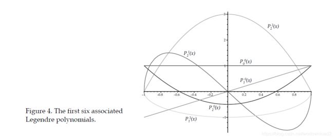The two arguments l and m break the family of polynomials into bands of functions where the argument
l is the band index and takes any positive integer value starting from 0, and the argument
m takes any integer value in the range [0,l].
Inside a band the polynomials are orthogonal w.r.t. a constant term and between bands they are orthogonal with a different constant. We can diagram this as a triangular grid of functions per band, giving us a total of n(n+1) coefficients for an n band approximation:
The process for evaluating Legendre polynomials turns out to be quite involved 相当复杂, which is why they’re rarely used for
approximating 1D functions.
The usual mathematical definition of the series is defined in terms of derivatives of imaginary numbers and requires a series of nasty cancellations of values that alternate in sign and this is not a floating point friendly process. Instead we turn to a set of recurrence relations (i.e. a recursive definition) that generate the current polynomial from earlier results in the series.

There are only three rules we need:

The main term of the recurrence takes the two previous bands l–1 and l–2 and generates a new higher band l from them.

The expression is the best place to start from as it is the only rule that needs no previous values. Note that x!! is the double factorial
function which, as (2m–1) is always odd, returns the product of all odd integers less than or equal to x. We can use P00(x) = 1 as the
initial state for an iterative loop that hoists us up from 0 to m.

This expression allows us to lift a term to a higher band.
The method for evaluating the function is first to try to generate the highest Pmm possible using rule 2, which if l=m is the final
answer. Since m the band until we meet the required l. We do this by calculating
Pm+1m using rule 3 only once (stopping if l=m+1) and finally
iterating rule 1 until the correct answer is found (noting that using
rule 1 has less floating point roundoff error than iterating rule 3).

double P(int l,int m,double x)
{
	// evaluate an Associated Legendre Polynomial P(l,m,x) at x
	double pmm = 1.0;
	if(m>0) 
	{
		double somx2 = sqrt((1.0-x)*(1.0+x));
		double fact = 1.0;
		for(int i=1; i<=m; i++) 
		{
			pmm *= (-fact) * somx2;
			fact += 2.0;
		}
	}
	if(l==m) return pmm;
	double pmmp1 = x * (2.0*m+1.0) * pmm;
	if(l==m+1) return pmmp1;
	double pll = 0.0;
	for(int ll=m+2; ll<=l; ++ll) 
	{
		pll = ( (2.0*ll-1.0)*x*pmmp1-(ll+m-1.0)*pmm ) / (ll-m);
		pmm = pmmp1;
		pmmp1 = pll;
	}
	return pll;
}

Spherical Harmonics
This is all fine for 1D functions, but what use is it on the 2D surface of a sphere? The associated Legendre polynomials are at
the heart of the Spherical Harmonics, a mathematical system analogous to the Fourier transform but defined across the surface
of a sphere.
The SH functions in general are defined on imaginary numbers but we are only interested in approximating real functions over the sphere (i.e. light intensity fields), so in this
document we will be working only with the Real Spherical
Harmonics. When we refer to an SH function we will only be
talking about the Real Spherical Harmonic functions.

Given the standard parameterization of points on the surface of a
unit sphere into spherical coordinates (which we will look at more
closely in a later section on coordinate systems):

the SH function is traditionally represented by the symbol y

where P is the same associated Legendre polynomials we look at earlier and K is just a scaling factor to normalize the functions:

In order to generate all the SH functions, the parameters l and m are defined slightly differently from the Legendre polynomials – l is still a positive integer starting from 0, but m takes signed integer values from –l to l.

Sometimes it is useful to think of the SH functions occurring in a
specific order so that we can flatten them into a 1D vector, so we
will also define the sequence yi

The code for evaluating an SH function looks like this:

double K(int l, int m)
{
	// renormalisation constant for SH function
	double temp = ((2.0*l+1.0)*factorial(l-m)) / (4.0*PI*factorial(l+m));
	return sqrt(temp);
}
double SH(int l, int m, double theta, double phi)
{
	// return a point sample of a Spherical Harmonic basis function
	// l is the band, range [0..N]
	// m in the range [-l..l]
	// theta in the range [0..Pi]
	// phi in the range [0..2*Pi]
	const double sqrt2 = sqrt(2.0);
	if(m==0) return K(l,0)*P(l,m,cos(theta));
	else if(m>0) return sqrt2*K(l,m)*cos(m*phi)*P(l,m,cos(theta));
	else return sqrt2*K(l,-m)*sin(-m*phi)*P(l,-m,cos(theta));
}

(Note: the fastest and most accurate way to implement
factorial(x) is as a table of precalculated floating point values.
You will never need more than 33 entries in the table.)

Traditionally, at about this point, papers using the SH functions like to show you tables of confusing polynomials, but I think it’s
more interesting to show what the functions actually look like when plotted as spherical functions.

Note how the first band is just a constant positive value – if you
render a self-shadowing model using just the 0-band coefficients
the resulting looks just like an accessibility shader with points
deep in crevices (high curvature) shaded darker than points on
flat surfaces. The l = 1 band coefficients cover signals that have
only one cycle per sphere and each one points along the x, y, or
z-axis and, as you will see later, linear combinations of just these
functions give us very good approximations to the cosine term in
the diffuse surface reflectance model.

SH Projection
The process for projecting a spherical function into SH coefficients is very simple.
To calculate a single coefficient for a specific band
you just integrate the product of your function f and the SH function y,
in effect working out how much your function is like
the basis function:

(Note: The equation above is very carefully written not to include
any mention of the parameterization we will use to generate
points on the surface of the sphere – the value s merely represents
some choice of a sample point. We will transform these equations
into concrete, parameterized versions that we can actually
calculate with in a moment, but for now we will stick with the
abstract idea of sample points over the sphere S.)
To reconstruct the approximated function (notated by f capped
with a tilde), we just take the reverse process and sum scaled
copies of the corresponding SH functions:

Now you can see why an n-th order approximation will require n2
coefficients. It can be proven that the true function f could be
reconstructed if we summed the infinite series of all SH
coefficients, so every reconstruction we will make will be an
approximation to the true function, technically known as a band–
limited approximation where band–limiting is just the process of
breaking a signal into it’s component frequencies and removing
frequencies higher than some threshold.

Let’s work through a concrete 混合 example of projecting a function
into SH coefficients using Monte Carlo integration.
First we need to decide on a parameterization of our sphere, so let’s use the
spherical coordinate system we defined earlier for the SH
functions. Let’s also choose a nice low-frequency function to
integrate so that we don’t have to generate too many coefficients to illustrate our point.
How about two large monochromatic light
sources at 90 degrees to each other and slightly rotated off-axis.
We’ll define these directly in spherical coordinates for now, but in
our full program we’ll be using a ray tracer to evaluate functions
like this directly from geometry.

Integrating some function f in spherical coordinates is done using
the formula:

(Why the sin(θ) in there? Remember that integration is all about
summing small patches of area on the surface of the sphere, and
the integral is just the limit as the edge lengths of these square
patches tend to zero. In this rectangular spherical coordinate
parameterization, patches around the equator are going to have
more effect on the final answer than the tiny patches around the
pole and the sin(θ) term encodes this effect. Don’t worry, it’s about
to disappear…)
Remember that to project a function into SH coefficients we want
to integrate the product of the function and an SH function so we
can write out our parameterised function for one coefficient as:

This equation is great for symbolic integration 符号积分 using a package like Mathematica or Maple, but we have to do this numerically.
We must evaluate this integral using Monte Carlo integration, so recalling the Monte Carlo estimator from earlier:

where xj is our array of pre-calculated samples and the function f is the product f(xj) = light(xj)yi(xj). As we have chosen all our samples to be unbiased w.r.t. area on the sphere, each sample has equal probability of appearing anywhere on the sphere giving us a probability function概率密度函数 of p(xj) = 1/4π and so a constant weighting function w(xj) = 1/p(xj) = 4π. Also, the use of unbiased 无偏采样 samples means that any other parameterization of the sphere would yield the same set of samples with the same probabilities, so we have magically factored out the parameterization of the sphere and our sin(θ) term disappears.

Using the SH_setup_spherical_samples function from earlier we can precalculate our jittered, unbiased set of samples and the SH coefficients for each band we want to SH project. Our integration code is then just a simple loop of multiply-accumulates into the correct elements of the SH vector, followed by a simple rescale of the results:

typedef double (*SH_polar_fn)(double theta, double phi);
void SH_project_polar_function(SH_polar_fn fn, const SHSample samples[], double result[])
{
	const double weight = 4.0*PI;
	// for each sample
	for(int i=0; i<n_samples; ++i) 
	{
		double theta = samples[i].sph.x;
		double phi = samples[i].sph.y;
		for(int n=0; n<n_coeff; ++n) 
		{
			result[n] += fn(theta,phi) * samples[i].coeff[n];
		}
	}
	// divide the result by weight and number of samples
	double factor = weight / n_samples;
	for(i=0; i<n_coeff; ++i) 
	{
		result[i] = result[i] * factor;
	}
}

Applying this process to the light source we defined earlier with 10,000 samples 一万个采样 over 4 bands gives us this vector of coefficients:

Reconstructing the SH functions for checking purposes from these 16 coefficients 15个呀呀呀 is simply a case of calculating a weighted sum of the basis functions:

giving us this low frequency approximated light source:

properties of SH functions
the SH functions have a bunch of interesting properties that make them more desirable for our purposes than other basis functions we could choose.
firstly, the SH functions are not just orthogonal but orthonomral, meaning if we integrate yiyj for any pair of i and j, the calculation will return 1 if i=j and 0 if i!=j.

the SH functions are also rotationally invariant, meaning that if a
function g is a rotated copy of function f, then, after SH projection it is true that:

in other words, SH projecting the rotated function g will give u exactly the same results as if u had rotated the input to f before SH projecting.
u are right, that is pretty confusing. it may not sound like such a big deal but this property is something that a lot of other compression methods can not claim, e.g. JPEG’s discrete consine transform encoding is not translation invariant which is what gives us the blocky look under high compression.

in practical terms it means that by using SH functions we can guarantee that when we animate scenes, move lights or rotate models, the intensity of lighting will not fluctuate波动，crawl, pulse, or have any other objectionable artifacts.

the next property is the killer one. we need to do lighting, so in general terms we will be taking some description of incoming illumination and multiplying it by some kind of decription of the surface reflectance (which we will be calling a transfer function) to get the resulting reflected light, but we need to do this over the entire sphere of incoming light. we need to integrate:

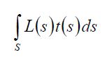
where L is the incomign light and t is the transfer function. if we project both the illumination and transfer functions into SH coefficients then orthogonality guarantees that the integral of the function’s products is the same as the dot product of their coefficients:

we have collapsed an integration over the sphere into a single dot product over the SH coefficients, just a series of multiply-adds. this is the key to the whole process——by projecting functions into SH space we can convert intergration over a sphere into a very fast operation.

this dot product returns a single scalar value which is the result of the integration, but there is another technique we can use for transforming SH functions. here is how the argument goes:

say we have some arbitrary spherical light source function a(s) that we do not know yet. we also have some shadowing function for a particular point on the surface b(s)
that describes how light at that point is shadowed (e.g. there is a nose above us that will block light coming from that direction), and we can evaluate it using a ray tracer. we want a way to transform the coefficients of the incoming light into another set of coefficients for a light that has been masked by the shadow function, and we will call the result c(s).
we can construct a linear operation that maps the SH projection of the shadowed light source c(s) using a transfer matrix without having to know the lighting function a(s).
to build the transfer matrix M, where each element of the matrix are indexed by i and j, the calculation is:

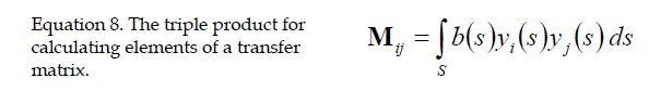
在a(s)不知道得情况下，也能实现构建好一个矩阵，次矩阵是b(s)和球谐函数得积分。

the result is a matric that we can use to transform from a light source into a shadowed light source using a simple matrix-vector multiply:

let us try an explicit example.
what would happen if we found a magic shadowing function that looks exactly like one of the SH functions; for example what if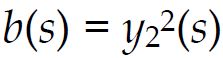
? this means we will be calcualting a triple product of SH functions:
不是四倍的吗？？？

the resulting matrix is mostly sparse稀疏的, and a plot of the non-zero elements in a 25x25 matrix looks like this:

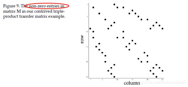
applying the matrix to the SH coefficients of a light source gives us another vector of SH coefficients,

the last property of SH functions is the most difficult to code, and probably the place where most people will get suck. we have asserted that SH functions are rotationally invariant, but how do we actually rotate an SH projected function? the answer is not simple. the first question to answer is “what form of rotation are u talking about?” do u want rotations in terms of Euler angles (α,β,γ), and if so which order of axes are u rotating about? XYZ, ZYX or ZYZ? how about specifying an axis and angle rotation by using a quaternion?
how about generalizing rotations into 3x3 rotation matrices with all the associated redundancy of symmetries? despite Sloan, Kautz and Snyder saying that SH functions are have “simple rotation”, they are not telling the whole story.

球谐函数的旋转不是那么容易的。

what we can say about the SH rotatoin process, from the rules of orthogonality, is that it is a linear operation and that coefficients between bands do not interact. in practical thems this means that we can rotate a vector of SH coefficients into another vector of SH coefficients into another vector of SH coefficients using a single n平方xn平方 rotation matrix and that the matrix will be block diagonal sparse, looking something like this:

so true, using the rotation operation could be seen as “a simple computation” once u have the rotation coefficients handy but constructing the rotation coefficients efficiently is far from simple.

as a quick aside 顺便提一下, let us look at another representation for the SH functions. so far we have been expressing SH functions in terms of spherical coordinates, but we can just as easily convert them to implicit functions on (x,y,z) by substituting in the spherical to Cartesian coordinate conversion formula and canceling out terms. doing so we come up with a surprisingly simple set of expressions:

to use these functions simply pick a point (x,y,z) on the unit sphere and crank it through the equation above to calcualte the SH coefficient in that direction. it is possible to use this form of equation for SH projection, but they turn out to be more useful to us as symbolic expressions.

we can build a rotation matrix for SH functions by building a matrix where each element is calculated using symbolic integrating of a rotated SH sample with an unrotated version:

一个旋转和一个不旋转

this will build a n平方xn平方 matrix of expressions that will map an unrotated vector of SH coefficients into a rotated one. for example, using the explicitly parameterised forumlation:

for the first three bands gives us a 9x9 matrix for rotating about the z-axis:

this matrix expands into higher bands as u would expect, with band N using the sine and cosine of Nα.

this technique looks greate for lower order SH functions——u simply decompose any rotation into a series of simpler rotations and recompose the results. in reality it quickly royal 皇家的 pain-in-the-ass for anything larger than a 2nd order SH function.

firstly, what is the minimum number of rotations we need to allow us transform an SH function to any possible orientation? if we use a ZYZ formulation we can get away with only two rotations, and one of them we already have the formula for! so, how to rotate about the y-axis? we can decompose it into a rotation of 90度 about the x-axis, a general rotation about the z-axis followed finally a rotation by -90度 about the x-axis. great, the x-axis rotation is a fixed angle fo we can just tabulate it as any array of constant floats:

taking a step back, let us look at the computational cost of this process. in matrix notation, we are calcualting:

that is 4 different 9x9 matrix multiplications, plus associated trig functions. given that cost of matrix-matrix multiplication is O(n三次方)，a naive implementation would use 2916 (9x9矩阵的相乘，每个元素需要计算9次的乘法，共有81个元素，所以需要4981=2916次乘法运算). mutiply adds. we can use the sparsity of the matrices to get this down to around 340 multiplies for a 5th order rotation, but it is not as cheap as it could be.

how about combining the rotations and multiplying throught the whole operations into one big explicit expression? for bands higher than 1 this turns out to produce some very scary trig expressions. here is the matrix for the first two bands:

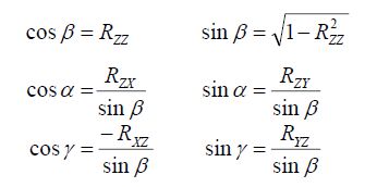
this matrix is useful for debugging, but to use it we have to convert our game engine to ZYZ rotations with all the associated gimbal lock problems when rotations end up aligning. was not this the reason we all converted to quaternions? there is a trick we can use to prevent us from entering this arena of pain and also speed up the calculation. one of the fundamental properties of rotation matrices in 3D is their numerous symmetries and we can exploit these to our advantage. given an ordinary 3x3 rotation matrix R:

we can reconstruct the trigonometric functions of the ZYZ euler angles (α,β,γ) directly using these identities:

now we have covered the properties of SH functions and coded up some tools
for manipulating them we can finally get to use them for generating some lighting for our models. we will go through a number of lighting techniques showing how each one is defined and how it is implemented.

let us assume we have already loaded a description of our polygonal model into an internal database. we are only interested in point sampling the world using a raytracer, so all we need is a list of vertices, normals and triangles. first we process the vertex-normal pairs into a set of unique “lighting points” by duplicating vertices