长短期记忆网络（LSTM）及其量化方法

长短期记忆网络（LSTM）

LSTM是一个比较常见的用于股市分析、序列数据预测的一种RNN网络。在1999年首次在[1]提出。源代码为改装自Github上某代码版本。

本文主要是通过复现单层LSTM的神经网络，使读者更加理解这样的一个过程。

Motivation

本文的Motivation：在研究过程中发现，有时需要调整网络的精度或要求内部变量被量化，一般来说我们用TFLite这样的工具去解决这种量化问题。而难受的事情是：TFLite并没有提供用于LSTM网络的模型！

那么唯一的解决方案：只能手打LSTM去解决。

Priciple

这里给出[1]的原理图。其实原著的原理图不是很好懂，看看接下来的公式或许能够增进理解。

看到这里还是啥都不明白？没关系！咱们结合代码一步步的看吧~
下面这个是更加友好的一个原理图（侵删）。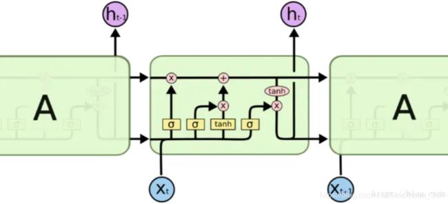

---

Code

numba
需要提一句，接下来会用到“@jit”的代码，是Python的加速模块numba的语句，经测试，能够显著提升for循环等带来的时间延缓，一个可供参考的数据就是：我的项目代码速度在加入numba模块的前后，是有提升三倍左右。

其它的说明
tanh函数和sigmoid函数在这里的量化过程中，也是按照某个量化函数来的。
具体函数表达式可以直接参考前半部分代码子函数tanh(x)和sigmoid(x)。

@jit
def tanh(x):
    #return np.tanh(x)
    nn,mm=x.shape
    for i in range(nn):
        for j in range(mm):
            if x[i,j]>1:
                x[i,j]=1
            elif x[i,j]<=-1:
                x[i,j]=-1
    return x
@jit
def softmax(x):
    e_x = np.exp(x - np.max(x))
    return e_x / e_x.sum(axis=0) 
@jit
def sigmoid1(x,mode=0):
    nn,mm=x.shape
    for i in range(nn):
        for j in range(mm):
            if x[i,j]>2:
                x[i,j]=1
            elif x[i,j]<=-2:
                x[i,j]=0
            else:
                x[i,j]=x[i,j]/4+0.5
    return x

---

LSTM元胞
这里姑且将cell翻译成元胞啦。
对于LSTM的内部前向传播过程（也就是通俗意义上的正向计算）呢，这里要分成五类，F,I,C,O,Y五个大类。
需要用到的变量：
x_concat，自变量x和前一元素状态a_pre的串接矩阵。
权重矩阵，刚刚说了有五类，那么权重矩阵就有五类。
偏置矩阵，显然也是有五类。
剩下的呢，就都是中间变量啦。
按顺序执行下面的公式即可，不解释原因（因为我也不能强行解释一些自己也很难理解的东西）。

需要解释一下，虚点是点积，也就是在线性代数里面所学到的矩阵乘法算法，要求矩阵列数等于另一个的行数；实点是对应相乘，也就要求两个矩阵行列数均完全一致。

@jit
def lstm_cell_forward(xt, a_prev, c_prev, parameters):
    """
    Implement a single forward step of the LSTM-cell as described in Figure (4)
    Arguments:
    xt -- your input data at timestep "t", numpy array of shape (n_x, m).
    a_prev -- Hidden state at timestep "t-1", numpy array of shape (n_a, m)
    c_prev -- Memory state at timestep "t-1", numpy array of shape (n_a, m)
    parameters -- python dictionary containing:
                        Wf -- Weight matrix of the forget gate, numpy array of shape (n_a, n_a + n_x)
                        bf -- Bias of the forget gate, numpy array of shape (n_a, 1)
                        Wi -- Weight matrix of the update gate, numpy array of shape (n_a, n_a + n_x)
                        bi -- Bias of the update gate, numpy array of shape (n_a, 1)
                        Wc -- Weight matrix of the first "tanh", numpy array of shape (n_a, n_a + n_x)
                        bc --  Bias of the first "tanh", numpy array of shape (n_a, 1)
                        Wo -- Weight matrix of the output gate, numpy array of shape (n_a, n_a + n_x)
                        bo --  Bias of the output gate, numpy array of shape (n_a, 1)
                        Wy -- Weight matrix relating the hidden-state to the output, numpy array of shape (n_y, n_a)
                        by -- Bias relating the hidden-state to the output, numpy array of shape (n_y, 1)
    Returns:
    a_next -- next hidden state, of shape (n_a, m)
    c_next -- next memory state, of shape (n_a, m)
    yt_pred -- prediction at timestep "t", numpy array of shape (n_y, m)
    cache -- tuple of values needed for the backward pass, contains (a_next, c_next, a_prev, c_prev, xt, parameters)
    Note: ft/it/ot stand for the forget/update/output gates, cct stands for the candidate value (c tilde),
          c stands for the memory value
    """

    # Retrieve parameters from "parameters"
    Wf = parameters["Wf"]
    bf = parameters["bf"]
    Wi = parameters["Wi"]
    bi = parameters["bi"]
    Wc = parameters["Wc"]
    bc = parameters["bc"]
    Wo = parameters["Wo"]
    bo = parameters["bo"]
    Wy = parameters["Wy"]
    by = parameters["by"]
   
    # Retrieve dimensions from shapes of xt and Wy
    n_x, m = xt.shape
    n_y, n_a = Wy.shape
    
    ### START CODE HERE ###
    # Concatenate a_prev and xt (≈3 lines)
    concat = np.zeros((n_x + n_a, m))
    concat[: n_a, :] = a_prev
    concat[n_a:, :] = xt
    # Compute values for ft, it, cct, c_next, ot, a_next using the formulas given figure (4) (≈6 lines)
    ft = sigmoid1(quantization(np.dot(Wf, concat) + bf))
    it = sigmoid1(quantization(np.dot(Wi, concat) + bi))
    cct = tanh(quantization(np.dot(Wc, concat) + bc))
    
    c_next = quantization(ft * c_prev + it * cct)
    
    ot = sigmoid1(quantization(np.dot(Wo, concat) + bo))
    
    a_next = quantization(ot * np.tanh(c_next))
    
    
    # Compute prediction of the LSTM cell (≈1 line)
    yt_pred = softmax(quantization(np.dot(Wy, a_next) + by))
    
    #quantization(yt_pred)
    ### END CODE HERE ###
    # store values needed for backward propagation in cache
    cache = (a_next, c_next, a_prev, c_prev, ft, it, cct, ot, xt, parameters)

    return a_next, c_next, yt_pred, cache

---

前向传播
实质是将上述元胞内的过程串接起来的作用，无需赘述。

# GRADED FUNCTION: lstm_forward
@jit
def lstm_forward(x, a0, parameters):
    """
    Implement the forward propagation of the recurrent neural network using an LSTM-cell described in Figure (3).
    Arguments:
    x -- Input data for every time-step, of shape (n_x, m, T_x).
    a0 -- Initial hidden state, of shape (n_a, m)
    parameters -- python dictionary containing:
                        Wf -- Weight matrix of the forget gate, numpy array of shape (n_a, n_a + n_x)
                        bf -- Bias of the forget gate, numpy array of shape (n_a, 1)
                        Wi -- Weight matrix of the update gate, numpy array of shape (n_a, n_a + n_x)
                        bi -- Bias of the update gate, numpy array of shape (n_a, 1)
                        Wc -- Weight matrix of the first "tanh", numpy array of shape (n_a, n_a + n_x)
                        bc -- Bias of the first "tanh", numpy array of shape (n_a, 1)
                        Wo -- Weight matrix of the output gate, numpy array of shape (n_a, n_a + n_x)
                        bo -- Bias of the output gate, numpy array of shape (n_a, 1)
                        Wy -- Weight matrix relating the hidden-state to the output, numpy array of shape (n_y, n_a)
                        by -- Bias relating the hidden-state to the output, numpy array of shape (n_y, 1)
    Returns:
    a -- Hidden states for every time-step, numpy array of shape (n_a, m, T_x)
    y -- Predictions for every time-step, numpy array of shape (n_y, m, T_x)
    caches -- tuple of values needed for the backward pass, contains (list of all the caches, x)
    """

    # Initialize "caches", which will track the list of all the caches
    caches = []

    ### START CODE HERE ###
    # Retrieve dimensions from shapes of x and Wy (≈2 lines)
    n_x, m, T_x = x.shape
    n_y, n_a = parameters["Wy"].shape

    # initialize "a", "c" and "y" with zeros (≈3 lines)
    a = np.zeros((n_a, m, T_x))
    c = np.zeros((n_a, m, T_x))
    y = np.zeros((n_y, m, T_x))

    # Initialize a_next and c_next (≈2 lines)
    a_next = a0
    c_next = np.zeros(a_next.shape)

    # loop over all time-steps
    for t in range(T_x):
        # Update next hidden state, next memory state, compute the prediction, get the cache (≈1 line)
        a_next, c_next, yt, cache = lstm_cell_forward(x[:, :, t], a_next, c_next, parameters)
        # Save the value of the new "next" hidden state in a (≈1 line)
        a[:, :, t] = a_next
        # Save the value of the prediction in y (≈1 line)
        y[:, :, t] = yt
        # Save the value of the next cell state (≈1 line)
        c[:, :, t] = c_next
        # Append the cache into caches (≈1 line)
        caches.append(cache)
    
    ### END CODE HERE ###

    # store values needed for backward propagation in cache
    caches = (caches, x)

    return a, y, c, caches

---

量化函数
代码中的quantization()函数是需要大家根据自己的需求进行补充的，你想对这个函数怎么操作，这一切都是看实际情况的。

---

Follow-up

下一篇会以Keras 2.0生成的模型为例，看看如何正确的调用已经训练好的权重和偏置矩阵，从而让上面的这个东西真正跑起来。

Reference

[1]Gers F A, Schmidhuber J, Cummins F. Learning to forget: Continual prediction with LSTM[J]. 1999.