C1W1-12_logistic-regression-cost-function

视频链接

Good see you again. In this optional video, you’re going to learn about the intuition behind the logistic regression cost function. Specifically, you will understand why the cost function is designed that way. You will see what happens when you predict the true label and you’ll see what happens, when you predict the wrong label. Let’s dive in and see how this logistic regression cost function is designed. Let’s have a look now at the equation of the cost function, while this might look like a big complicated equation, it’s actually rather straightforward, once you break it down into its components.

很高兴再次见到你。在这个可选的视频中，你将会学到逻辑回归成本函数背后的直觉。具体来讲，你将会理解为什么成本函数设计成那种方式。你将会看到你预测出正确的标签会发生什么，当你预测出错误的标签又会发生什么。让我们一探究竟，看看逻辑回归成本函数是怎么设计的。现在让我们看下成本函数的方程，这可能看起来像一个大的复杂的方程，一旦你把它分解成它的各个组件，其实就很简单了。

First, have a look at the left hand side of the equation where you find a sum over the variable m, which is just the number of training example in your training set. This indicates that you’re going to sum over the cost of each training example. Out front, there is a -1/m, indicating that when combined with the sum, this will be some kind of average. The minus sign ensures that your overall costs will always be a positive number as you’ll see clearly later in this video. Inside the square brackets, the equation has two terms that are added together. To consider what each of these terms contribute to the cost function for each training example, let’s have a look at each of them separately. The term on the left is the product of y superscript i, which is the label for each training example, most applied by the log of the prediction, which is the logistic regression function applied to each training example. Represented as h of superscript i, and a parameter theta. Now, consider the case when your label is 0. In this case, the function h can return any value, and the entire term will be 0 because 0 times anything is just 0. What about the case when your label is 1? If your prediction is close to 1, the the log of your prediction will be close to 0, because, as you may recall, the log of 1 is 0. And the product will also be near 0. If your label is 1, and your prediction is close to 0, then this term blows up and approaches negative infinity. Intuitively, now, you can see that this is the relevant term in your cost function when your label is 1. When your prediction is close to the label value, the loss is small, and when your label and prediction disagree, the overall cost goes up.

首先看下等式的左边，你可以找到变量m的和，它是训练集中的训练样本数。这表明你将对每个训练样本的成本进行求和。前面有一个-1/m，表明与总和结合时，这将是某种平均值。这个负号确保你的总成本总是一个正数，在这个视频的后面你会清楚的看到。在方括号里面，这个方程有两项加在一起。为了考虑这些条件对每个训练样本的成本函数的贡献，让我们分开来看它们的每一项。左边的这项是$y^i$的乘积,是每个训练样本的标签，大多数应用于预测的对数，它是应用在每个训练样本上的逻辑回归函数。表示为$h^i$,和一个参数$\theta$。现在考虑当你的标签是0的这种情况。在这种情况下，函数h返回任意值，整个项是0，因为0乘任何数都为0。当标签为1时是什么样一种情况呢？如果你的预测接近1，你的预测的对数接近于0，因为你可能记得，1的对数是0。乘积也将接近0。如果你的标签是1，你的预测接近0，然后这一项膨胀，趋近负无穷。现在你能直观地看到当你的标签为1时这是成本函数中的相关项。当你的预测接近标签值是，损失是小的，当你的标签和预测不一致是，总成本就会上升。

Now consider the term on the right hand side of the cost function equation, in this case, if your label is 1, then the 1-y term goes to 0. And so any value returned by the logistic regression function will result in a 0 for the entire term, because again, 0 times anything is just 0. If your label is 0, and the logistic regression function returns a value close to 0, then the products in this term will again be close to 0. If on the other hand your label is 0 and your prediction is close to 1, then the log term will blow up and the overall term will approach to negative infinity.

现在考虑成本函数方程的右手边这项。在这种情况下，如果你的标签是1，然后1-y项趋于0。所以逻辑回归函数所有值返回的结果在这一项中是0，又因为，0乘以任意值始终为0。如果你的标签是0，逻辑回归函数返回一个趋于0的值，然后这项中的乘积将有一次接近于0。另一方面，如果你的标签是0，你的预测接近于1，然后这项的对象将膨胀，整个项将会趋于负无穷。

From this exercise you can see now that there is one term in the cost function that is relevant when your label is 0, and another that is relevant when the label is 1. In each of these terms, you’re taking the log of a value between 0 and 1, which will always return a negative number, and so the minus sign out front ensures that the overall cost will always be a positive number. Now, let’s have a look at what the cost function looks like for each of the labels. 0 and 1, overall possible prediction values.

从这个练习中，你现在能够看到当你的标签为0时，在成本函数中有一项是相关的，当标签为1时，另一项相关。在每一项中，取到一个0到1的对数，这将会返回一个负值，所以前面的负号确保总成本将总是一个正数。现在让我们看下每个标签的成本函数是怎样的。0到1之间总体可能的预测值。

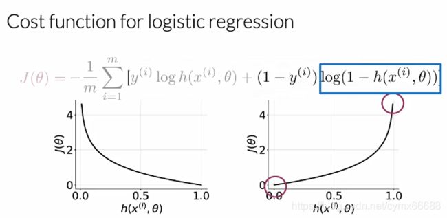
First, we’re going to look at the loss when the label is 1. In this plot, you have your prediction value on the horizontal axis and the cost associated with a single training example on the vertical axis. In this case J, of theta simplifies to just negative log h(x(theta)). When your prediction is close to 1, the loss is close to 0. Because your prediction agrees well with the label. And when the prediction is close to 0, the loss approaches infinity, because your prediction and the label disagree strongly. The opposite is true when the label is 0. In this case J(theta) reduces to just minus log(1-h(x, theta)). Now when your prediction is close to 0, the loss is also close to 0. And when your prediction is close to 1, the loss approaches infinity.

首先我们看下当标签为1时的损失。在这个图里，横轴是预测值，纵轴是与单个简单训练样本相关的成本。在这种情况下J，简化为$-lo{g}_h(x(\theta ))$。当你的预测接近于1，损失接近0。因为你的预测和标签很一致。当预测接近于0，损失接近无穷，因为你的预测和标签非常不一致。当标签为0时，相反为真。在这种情况下$J(\theta )$化简为$-log(1-h(x,\theta ))$。现在当你的预测接近于0时，损失也接近于0。当你的预测接近于1时，损失接近于无穷大。

You now understand how the logistic regression cost function works. You saw what happened when you predicted a 1 and the true label was a 1. You also saw what happened when you predicted a 0, and the true label was a 0. In the next week, you will learn about Naive Bayes, which is a different types of classification algorithm, which also allows you to predict whether a tweet is positive or negative.

你现在理解了逻辑回归成本函数是如何起作用的。你能知道当你预测一个1,真实标签是1时，发生了什么。你也知道当你预测一个0，真实标签是一个0时发生了什么。在下周，你将学习贝叶斯，一种不同类型的分类算法，它还允许你预测推特是积极的还是消极的。