Tensorflow2.1.0 基础线性回归

样例为《概率论与数理统计》中线性回归一节中的例子

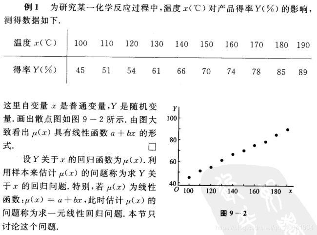
我们希望通过对该数据进行线性回归，即使用线性模型 来拟合上述数据，此处 a 和 b 是待求的参数

接下来，我们使用梯度下降方法来求线性模型中两个参数 a 和 b 的值 3。

回顾机器学习的基础知识，对于多元函数 求局部极小值，梯度下降 的过程如下：

• 初始化自变量为 ， k=0

• 迭代进行下列步骤直到满足收敛条件：

  • 求函数 关于自变量的梯度

  • 更新自变量： 。这里 是学习率（也就是梯度下降一次迈出的 “步子” 大小）

  • k <- k+1

接下来，我们考虑如何使用程序来实现梯度下降方法，求得线性回归的解 。

 

NumPy下的线性回归

# 导入相应的模块
import tensorflow as tf
import numpy as np

# 定义数据，并进行归一化操作
X_raw = np.array([100, 110, 120, 130, 140, 150, 160, 170, 180, 190], dtype=np.float32)
y_raw = np.array([45, 51, 54, 61, 66, 70, 74, 78, 85, 89], dtype=np.float32)

x = (X_raw) / 100.
y = (y_raw) / 100.

a, b = 0, 0

num_epoch = 5000
learning_rate = 1e-3
print(learning_rate)
for i in range(num_epoch):
    # 预测值
    y_pred = a * x + b
    # 损失函数为reduce_sum(reduce_squre(y_pred-y))
    # 分别计算损失函数对a,b的偏导数
    grad_a, grad_b = (y_pred - y).dot(x), (y_pred - y).sum()
    # 更新参数
    a, b = a-learning_rate*grad_a, b-learning_rate*grad_b
    # print(i, 'grad_a:', grad_a, ', grad_b:', grad_b, ', a:', a, ', b:', b)

print(a,b)

TensorFLow下的线性回归

import tensorflow as tf
import numpy as np

X_raw = np.array([100, 110, 120, 130, 140, 150, 160, 170, 180, 190], dtype=np.float32)
y_raw = np.array([45, 51, 54, 61, 66, 70, 74, 78, 85, 89], dtype=np.float32)

x = (X_raw) / 20.
y = (y_raw) / 20.

X = tf.constant(x)
Y = tf.constant(y)

a = tf.Variable(initial_value=0.)
b = tf.Variable(initial_value=0.)
variables = [a, b]

num_epoch = 50

# 声明keras模块下的随机梯度优化算法，学习率为0.001
optimizer = tf.keras.optimizers.SGD(learning_rate=1e-3)
for e in range(num_epoch):
    with tf.GradientTape() as tape:
        y_pred = a*X+b
        loss = tf.reduce_mean(tf.square(y_pred-Y))

    # 计算损失函数对参数的偏导数
    grads = tape.gradient(loss, variables)
    # 更新参数
    optimizer.apply_gradients(grads_and_vars=zip(grads, variables))

print(a,b)