睿智的目标检测46——Pytorch搭建自己的Centernet目标检测平台
睿智的目标检测46——Pytorch搭建自己的Centernet目标检测平台
- 学习前言
- 什么是Centernet目标检测算法
- 源码下载
- Centernet实现思路
-
- 一、预测部分
-
- 1、主干网络介绍
- 2、利用初步特征获得高分辨率特征图
- 3、Center Head从特征获取预测结果
- 4、预测结果的解码
- 5、在原图上进行绘制
- 二、训练部分
-
- 1、真实框的处理
- 2、利用处理完的真实框与对应图片的预测结果计算loss
- 训练自己的Centernet模型
学习前言
Pytorch版本的实现也要做一下。

什么是Centernet目标检测算法

如今常见的目标检测算法通常使用先验框的设定,即先在图片上设定大量的先验框,网络的预测结果会对先验框进行调整获得预测框,先验框很大程度上提高了网络的检测能力,但是也会收到物体尺寸的限制。
Centernet采用不同的方法,构建模型时将目标作为一个点——即目标BBox的中心点。
Centernet的检测器采用关键点估计来找到中心点,并回归到其他目标属性。
论文中提到:模型是端到端可微的,更简单,更快,更精确。Centernet的模型实现了速度和精确的很好权衡。
源码下载
https://github.com/bubbliiiing/centernet-pytorch
喜欢的可以点个star噢。
Centernet实现思路
一、预测部分
1、主干网络介绍
Centernet用到的主干特征网络有多种,一般是以Hourglass Network、DLANet或者Resnet为主干特征提取网络,由于centernet所用到的Hourglass Network参数量太大,有19000W参数,DLANet并没有keras资源,本文以Resnet为例子进行解析。
ResNet50有两个基本的块,分别名为Conv Block和Identity Block,其中Conv Block输入和输出的维度是不一样的,所以不能连续串联,它的作用是改变网络的维度;Identity Block输入维度和输出维度相同,可以串联,用于加深网络的。
Conv Block的结构如下:

Identity Block的结构如下:

这两个都是残差网络结构。
当我们输入的图片是512x512x3的时候,整体的特征层shape变化为:
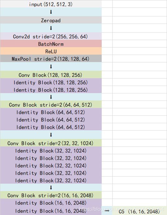
我们取出最终一个block的输出进行下一步的处理。也就是图上的C5,它的shape为16x16x2048。利用主干特征提取网络,我们获取到了一个初步的特征层,其shape为16x16x2048。
from __future__ import absolute_import
from __future__ import division
from __future__ import print_function

import pdb
import math
import torch
import torch.nn as nn
import torch.nn.functional as F
import torch.utils.model_zoo as model_zoo
from torchvision.models.utils import load_state_dict_from_url
from torch.autograd import Variable


model_urls = {

'resnet18': 'https://s3.amazonaws.com/pytorch/models/resnet18-5c106cde.pth',
'resnet34': 'https://s3.amazonaws.com/pytorch/models/resnet34-333f7ec4.pth',
'resnet50': 'https://s3.amazonaws.com/pytorch/models/resnet50-19c8e357.pth',
'resnet101': 'https://s3.amazonaws.com/pytorch/models/resnet101-5d3b4d8f.pth',
'resnet152': 'https://s3.amazonaws.com/pytorch/models/resnet152-b121ed2d.pth',
}


class Bottleneck(nn.Module):
    expansion = 4

    def __init__(self, inplanes, planes, stride=1, downsample=None):
        super(Bottleneck, self).__init__()
        self.conv1 = nn.Conv2d(inplanes, planes, kernel_size=1, stride=stride, bias=False) # change
        self.bn1 = nn.BatchNorm2d(planes)
        self.conv2 = nn.Conv2d(planes, planes, kernel_size=3, stride=1, # change
                    padding=1, bias=False)
        self.bn2 = nn.BatchNorm2d(planes)
        self.conv3 = nn.Conv2d(planes, planes * 4, kernel_size=1, bias=False)
        self.bn3 = nn.BatchNorm2d(planes * 4)
        self.relu = nn.ReLU(inplace=True)
        self.downsample = downsample
        self.stride = stride

    def forward(self, x):
        residual = x

        out = self.conv1(x)
        out = self.bn1(out)
        out = self.relu(out)

        out = self.conv2(out)
        out = self.bn2(out)
        out = self.relu(out)

        out = self.conv3(out)
        out = self.bn3(out)

        if self.downsample is not None:
            residual = self.downsample(x)

        out += residual
        out = self.relu(out)

        return out


class ResNet(nn.Module):
    def __init__(self, block, layers, num_classes=1000):
        self.inplanes = 64
        super(ResNet, self).__init__()
        self.conv1 = nn.Conv2d(3, 64, kernel_size=7, stride=2, padding=3,bias=False)
        self.bn1 = nn.BatchNorm2d(64)
        self.relu = nn.ReLU(inplace=True)
        self.maxpool = nn.MaxPool2d(kernel_size=3, stride=2, padding=0, ceil_mode=True) # change
        self.layer1 = self._make_layer(block, 64, layers[0])
        self.layer2 = self._make_layer(block, 128, layers[1], stride=2)
        self.layer3 = self._make_layer(block, 256, layers[2], stride=2)
        self.layer4 = self._make_layer(block, 512, layers[3], stride=2)

        self.avgpool = nn.AvgPool2d(7)
        self.fc = nn.Linear(512 * block.expansion, num_classes)

        for m in self.modules():
            if isinstance(m, nn.Conv2d):
                n = m.kernel_size[0] * m.kernel_size[1] * m.out_channels
                m.weight.data.normal_(0, math.sqrt(2. / n))
            elif isinstance(m, nn.BatchNorm2d):
                m.weight.data.fill_(1)
                m.bias.data.zero_()

    def _make_layer(self, block, planes, blocks, stride=1):
        downsample = None
        if stride != 1 or self.inplanes != planes * block.expansion:
            downsample = nn.Sequential(
                nn.Conv2d(self.inplanes, planes * block.expansion,
                    kernel_size=1, stride=stride, bias=False),
            nn.BatchNorm2d(planes * block.expansion),
        )

        layers = []
        layers.append(block(self.inplanes, planes, stride, downsample))
        self.inplanes = planes * block.expansion
        for i in range(1, blocks):
            layers.append(block(self.inplanes, planes))

        return nn.Sequential(*layers)

    def forward(self, x):
        x = self.conv1(x)
        x = self.bn1(x)
        x = self.relu(x)
        x = self.maxpool(x)

        x = self.layer1(x)
        x = self.layer2(x)
        x = self.layer3(x)
        x = self.layer4(x)

        x = self.avgpool(x)
        x = x.view(x.size(0), -1)
        x = self.fc(x)

        return x

def resnet50(pretrain = True):
    model = ResNet(Bottleneck, [3, 4, 6, 3])

    if pretrain:
        state_dict = load_state_dict_from_url(model_urls['resnet50'])
        model.load_state_dict(state_dict)

    # 获取特征提取部分
    features = list([model.conv1, model.bn1, model.relu, model.maxpool, model.layer1, model.layer2, model.layer3, model.layer4])
    features = nn.Sequential(*features)
    return features
2、利用初步特征获得高分辨率特征图

利用上一步获得到的resnet50的最后一个特征层的shape为(16,16,2048)。
对于该特征层,centernet利用三次反卷积进行上采样,从而更高的分辨率输出。为了节省计算量,这3个反卷积的输出通道数分别为256,128,64。
每一次反卷积,特征层的高和宽会变为原来的两倍,因此,在进行三次反卷积上采样后,我们获得的特征层的高和宽变为原来的8倍,此时特征层的高和宽为128x128,通道数为64。
此时我们获得了一个128x128x64的有效特征层(高分辨率特征图),我们会利用该有效特征层获得最终的预测结果。
实现代码如下:
#---------------------------------------#
#   进行三次上采样
#---------------------------------------#
class Decoder(nn.Module):
    def __init__(self, inplanes, bn_momentum=0.1):
        super(Decoder, self).__init__()
        self.bn_momentum = bn_momentum

        self.inplanes = inplanes
        self.deconv_with_bias = False
        # 16, 16, 2048  ->  32, 32, 256 -> 64, 64, 128 -> 128, 128, 64
        self.deconv_layers = self._make_deconv_layer(
            num_layers=3,
            num_filters=[256, 128, 64],
            num_kernels=[4, 4, 4],
        )

    def _make_deconv_layer(self, num_layers, num_filters, num_kernels):
        layers = []
        for i in range(num_layers):
            kernel = num_kernels[i]
            planes = num_filters[i]

            layers.append(
                nn.ConvTranspose2d(
                    in_channels=self.inplanes,
                    out_channels=planes,
                    kernel_size=kernel,
                    stride=2,
                    padding=1,
                    output_padding=0,
                    bias=self.deconv_with_bias))
            layers.append(nn.BatchNorm2d(planes, momentum=self.bn_momentum))
            layers.append(nn.ReLU(inplace=True))
            self.inplanes = planes
        return nn.Sequential(*layers)

    def forward(self, x):
        return self.deconv_layers(x)
3、Center Head从特征获取预测结果
通过上一步我们可以获得一个128x128x64的高分辨率特征图。
这个特征层相当于将整个图片划分成128x128个区域,每个区域存在一个特征点,如果某个物体的中心落在这个区域,那么就由这个特征点来确定。
(某个物体的中心落在这个区域,则由这个区域左上角的特征点来约定)
我们可以利用这个特征层进行三个卷积,分别是:
1、热力图预测,此时卷积的通道数为num_classes,最终结果为(128,128,num_classes),代表每一个热力点是否有物体存在,以及物体的种类;
2、中心点预测,此时卷积的通道数为2,最终结果为(128,128,2),代表每一个物体中心距离热力点偏移的情况;
3、宽高预测,此时卷积的通道数为2,最终结果为(128,128,2),代表每一个物体宽高的预测情况;
实现代码为:
#---------------------------------------#
#   CenterHead
#   利用特征层获得最终的预测结果
#---------------------------------------#
class Head(nn.Module):
    def __init__(self, num_classes=80, out_channel=64, bn_momentum=0.1):
        super(Head, self).__init__()

        self.cls_head = nn.Sequential(
            nn.Conv2d(64, out_channel,
                      kernel_size=3, padding=1, bias=False),
            nn.BatchNorm2d(out_channel, momentum=bn_momentum),
            nn.ReLU(inplace=True),
            nn.Conv2d(out_channel, num_classes,
                      kernel_size=1, stride=1, padding=0))
        self.wh_head = nn.Sequential(
            nn.Conv2d(64, out_channel,
                      kernel_size=3, padding=1, bias=False),
            nn.BatchNorm2d(out_channel, momentum=bn_momentum),
            nn.ReLU(inplace=True),
            nn.Conv2d(out_channel, 2,
                      kernel_size=1, stride=1, padding=0))
        self.reg_head = nn.Sequential(
            nn.Conv2d(64, out_channel,
                      kernel_size=3, padding=1, bias=False),
            nn.BatchNorm2d(out_channel, momentum=bn_momentum),
            nn.ReLU(inplace=True),
            nn.Conv2d(out_channel, 2,
                      kernel_size=1, stride=1, padding=0))

    def forward(self, x):
        hm = self.cls_head(x).sigmoid_()
        wh = self.wh_head(x)
        offset = self.reg_head(x)
        return hm, wh, offset
4、预测结果的解码
在对预测结果进行解码之前,我们再来看看预测结果代表了什么,预测结果可以分为3个部分:
1、heatmap热力图预测,此时卷积的通道数为num_classes,最终结果为(128,128,num_classes),代表每一个热力点是否有物体存在,以及物体的种类,最后一维度num_classes中的预测值代表属于每一个类的概率;
2、reg中心点预测,此时卷积的通道数为2,最终结果为(128,128,2),代表每一个物体中心距离热力点偏移的情况,最后一维度2中的预测值代表当前这个特征点向右下角偏移的情况;
3、wh宽高预测,此时卷积的通道数为2,最终结果为(128,128,2),代表每一个物体宽高的预测情况,最后一维度2中的预测值代表当前这个特征点对应的预测框的宽高;
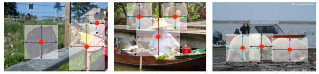
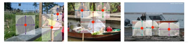
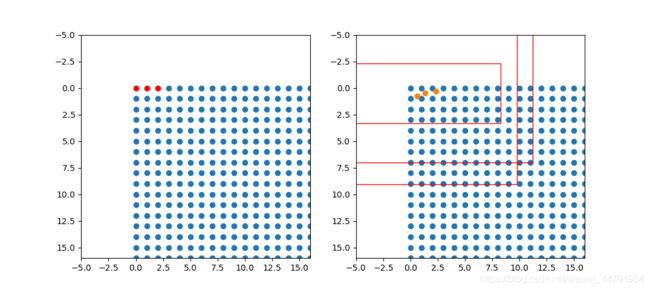
特征层相当于将图像划分成128x128个特征点每个特征点负责预测中心落在其右下角一片区域的物体。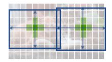
如图所示,蓝色的点为128x128的特征点,此时我们对左图红色的三个点进行解码操作演示:
1、进行中心点偏移,利用reg中心点预测对特征点坐标进行偏移,左图红色的三个特征点偏移后是右图橙色的三个点;
2、利用中心点加上和减去 wh宽高预测结果除以2,获得预测框的左上角和右下角。
3、此时获得的预测框就可以绘制在图片上了。
除去这样的解码操作,还有非极大抑制的操作需要进行,防止同一种类的框的堆积。
在论文中所说,centernet不像其它目标检测算法,在解码之后需要进行非极大抑制,centernet的非极大抑制在解码之前进行。采用的方法是最大池化,利用3x3的池化核在热力图上搜索,然后只保留一定区域内得分最大的框。
在实际使用时发现,当目标为小目标时,确实可以不在解码之后进行非极大抑制的后处理,如果目标为大目标,网络无法正确判断目标的中心时,还是需要进行非击大抑制的后处理的。
def pool_nms(hm, pool_size=3):
    pad = (pool_size - 1) // 2
    hm_max = F.max_pool2d(hm, pool_size, stride=1, padding=pad)
    keep = (hm_max == hm).float()
    return hm * keep

def decode_bbox(pred_hms, pred_whs, pred_offsets, image_size, threshold, cuda, topk=100):
    pred_hms = pool_nms(pred_hms)

    h, w = image_size[0], image_size[1]
    b, c, output_h, output_w = pred_hms.shape
    detects = []
    for batch in range(b):
        heat_map    = pred_hms[batch].permute(1,2,0).view([-1,c])
        pred_wh     = pred_whs[batch].permute(1,2,0).view([-1,2])
        pred_offset = pred_offsets[batch].permute(1,2,0).view([-1,2])

        yv, xv = torch.meshgrid(torch.arange(0, output_w), torch.arange(0, output_h))

        xv, yv = xv.flatten().float(), yv.flatten().float()
        if cuda:
            xv = xv.cuda()
            yv = yv.cuda()

        class_conf, class_pred = torch.max(heat_map, dim=-1)
        mask = class_conf > threshold

        pred_wh_mask = pred_wh[mask]
        pred_offset_mask = pred_offset[mask]
        if len(pred_wh_mask)==0:
            detects.append([])
            continue
        xv_mask = torch.unsqueeze(xv[mask] + pred_offset_mask[..., 0],-1)
        yv_mask = torch.unsqueeze(yv[mask] + pred_offset_mask[..., 1],-1)

        half_w, half_h = pred_wh_mask[..., 0:1] / 2, pred_wh_mask[..., 1:2] / 2
        bboxes = torch.cat([xv_mask - half_w, yv_mask - half_h, xv_mask + half_w, yv_mask + half_h], dim=1)
        bboxes[:, [0, 2]] *= w / output_w
        bboxes[:, [1, 3]] *= h / output_h

        detect = torch.cat([bboxes,torch.unsqueeze(class_conf[mask],-1),torch.unsqueeze(class_pred[mask],-1).float()],dim=-1)

        arg_sort = torch.argsort(detect[:,-2], descending=True)
        detect = detect[arg_sort]

        detects.append(detect.cpu().numpy()[:topk])
    return detects
5、在原图上进行绘制
通过第三步,我们可以获得预测框在原图上的位置,而且这些预测框都是经过筛选的。这些筛选后的框可以直接绘制在图片上,就可以获得结果了。
二、训练部分
1、真实框的处理
既然在centernet中,物体的中心落在哪个特征点的右下角就由哪个特征点来负责预测,那么在训练的时候我们就需要找到真实框和特征点之间的关系。
真实框和特征点之间的关系,对应方式如下:
1、找到真实框的中心,通过真实框的中心找到其对应的特征点。
2、根据该真实框的种类,对网络应该有的热力图进行设置,即heatmap热力图。其实就是将对应的特征点里面的对应的种类,它的中心值设置为1,然后这个特征点附近的其它特征点中该种类对应的值按照高斯分布不断下降。

3、除去heatmap热力图外,还需要设置特征点对应的reg中心点和wh宽高,在找到真实框对应的特征点后,还需要设置该特征点对应的reg中心和wh宽高。这里的reg中心和wh宽高都是对于128x128的特征层的。
4、在获得网络应该有的预测结果后,就可以将预测结果和应该有的预测结果进行对比,对网络进行反向梯度调整了。
实现代码如下:
class Generator(object):
    def __init__(self,batch_size,train_lines,val_lines,
                input_size,num_classes):

        self.batch_size = batch_size
        self.train_lines = train_lines
        self.val_lines = val_lines
        self.input_size = input_size
        self.output_size = (int(input_size[0]/4) , int(input_size[1]/4))
        self.num_classes = num_classes

    def get_random_data(self, annotation_line, input_shape, random=True, jitter=.3, hue=.1, sat=1.5, val=1.5, proc_img=True):
        '''r实时数据增强的随机预处理'''
        line = annotation_line.split()
        image = Image.open(line[0])
        iw, ih = image.size
        h, w = input_shape
        box = np.array([np.array(list(map(int,box.split(',')))) for box in line[1:]])

        # resize image
        new_ar = w/h * rand(1-jitter,1+jitter)/rand(1-jitter,1+jitter)
        scale = rand(0.5, 1.5)
        if new_ar < 1:
            nh = int(scale*h)
            nw = int(nh*new_ar)
        else:
            nw = int(scale*w)
            nh = int(nw/new_ar)
        image = image.resize((nw,nh), Image.BICUBIC)

        # place image
        dx = int(rand(0, w-nw))
        dy = int(rand(0, h-nh))
        new_image = Image.new('RGB', (w,h), (128,128,128))
        new_image.paste(image, (dx, dy))
        image = new_image

        # flip image or not
        flip = rand()<.5
        if flip: image = image.transpose(Image.FLIP_LEFT_RIGHT)

        # distort image
        hue = rand(-hue, hue)
        sat = rand(1, sat) if rand()<.5 else 1/rand(1, sat)
        val = rand(1, val) if rand()<.5 else 1/rand(1, val)
        x = cv2.cvtColor(np.array(image,np.float32)/255, cv2.COLOR_RGB2HSV)
        x[..., 0] += hue*360
        x[..., 0][x[..., 0]>1] -= 1
        x[..., 0][x[..., 0]<0] += 1
        x[..., 1] *= sat
        x[..., 2] *= val
        x[x[:,:, 0]>360, 0] = 360
        x[:, :, 1:][x[:, :, 1:]>1] = 1
        x[x<0] = 0
        image_data = cv2.cvtColor(x, cv2.COLOR_HSV2RGB)*255

        # correct boxes
        box_data = np.zeros((len(box),5))
        if len(box)>0:
            np.random.shuffle(box)
            box[:, [0,2]] = box[:, [0,2]]*nw/iw + dx
            box[:, [1,3]] = box[:, [1,3]]*nh/ih + dy
            if flip: box[:, [0,2]] = w - box[:, [2,0]]
            box[:, 0:2][box[:, 0:2]<0] = 0
            box[:, 2][box[:, 2]>w] = w
            box[:, 3][box[:, 3]>h] = h
            box_w = box[:, 2] - box[:, 0]
            box_h = box[:, 3] - box[:, 1]
            box = box[np.logical_and(box_w>1, box_h>1)] # discard invalid box
            box_data = np.zeros((len(box),5))
            box_data[:len(box)] = box
        if len(box) == 0:
            return image_data, []

        if (box_data[:,:4]>0).any():
            return image_data, box_data
        else:
            return image_data, []

    def generate(self, train=True):
        while True:
            if train:
                # 打乱
                shuffle(self.train_lines)
                lines = self.train_lines
            else:
                shuffle(self.val_lines)
                lines = self.val_lines
            batch_images = np.zeros((self.batch_size, self.input_size[2], self.input_size[0], self.input_size[1]), dtype=np.float32)

            batch_hms = np.zeros((self.batch_size, self.output_size[0], self.output_size[1], self.num_classes),
                                dtype=np.float32)
            batch_whs = np.zeros((self.batch_size, self.output_size[0], self.output_size[1], 2), dtype=np.float32)
            batch_regs = np.zeros((self.batch_size, self.output_size[0], self.output_size[1], 2), dtype=np.float32)
            batch_reg_masks = np.zeros((self.batch_size, self.output_size[0], self.output_size[1]), dtype=np.float32)

            b = 0
            for annotation_line in lines:
                img,y=self.get_random_data(annotation_line,self.input_size[0:2])

                if len(y)==0:
                    continue
                boxes = np.array(y[:,:4],dtype=np.float32)
                boxes[:,0] = boxes[:,0]/self.input_size[1]*self.output_size[1]
                boxes[:,1] = boxes[:,1]/self.input_size[0]*self.output_size[0]
                boxes[:,2] = boxes[:,2]/self.input_size[1]*self.output_size[1]
                boxes[:,3] = boxes[:,3]/self.input_size[0]*self.output_size[0]
                if ((boxes[:,3]-boxes[:,1])<=0).any() and ((boxes[:,2]-boxes[:,0])<=0).any():
                    continue

                for i in range(boxes.shape[0]):
                    bbox = boxes[i].copy()
                    bbox = np.array(bbox)
                    bbox[[0, 2]] = np.clip(bbox[[0, 2]], 0, self.output_size[1] - 1)
                    bbox[[1, 3]] = np.clip(bbox[[1, 3]], 0, self.output_size[0] - 1)
                    cls_id = int(y[i,-1])

                    h, w = bbox[3] - bbox[1], bbox[2] - bbox[0]
                    if h > 0 and w > 0:
                        radius = gaussian_radius((math.ceil(h), math.ceil(w)))
                        radius = max(0, int(radius))
                        ct = np.array([(bbox[0] + bbox[2]) / 2, (bbox[1] + bbox[3]) / 2], dtype=np.float32)
                        ct_int = ct.astype(np.int32)
                        batch_hms[b, :, :, cls_id] = draw_gaussian(batch_hms[b, :, :, cls_id], ct_int, radius)

                        batch_whs[b, ct_int[1], ct_int[0]] = 1. * w, 1. * h
                        batch_regs[b, ct_int[1], ct_int[0]] = ct - ct_int
                        batch_reg_masks[b, ct_int[1], ct_int[0]] = 1

                batch_images[b] = np.transpose(preprocess_image(img), (2, 0, 1))
                b = b + 1
                if b == self.batch_size:
                    b = 0
                    yield batch_images, batch_hms, batch_whs, batch_regs, batch_reg_masks
                    batch_images = np.zeros((self.batch_size, self.input_size[2], self.input_size[0], self.input_size[1]), dtype=np.float32)

                    batch_hms = np.zeros((self.batch_size, self.output_size[0], self.output_size[1], self.num_classes),
                                        dtype=np.float32)
                    batch_whs = np.zeros((self.batch_size, self.output_size[0], self.output_size[1], 2), dtype=np.float32)
                    batch_regs = np.zeros((self.batch_size, self.output_size[0], self.output_size[1], 2), dtype=np.float32)
                    batch_reg_masks = np.zeros((self.batch_size, self.output_size[0], self.output_size[1]), dtype=np.float32)
2、利用处理完的真实框与对应图片的预测结果计算loss
loss计算分为三个部分,分别是:
1、热力图的loss
2、reg中心点的loss
3、wh宽高的loss
具体情况如下:
1、热力图的loss采用focal loss的思想进行运算,其中 α 和 β 是Focal Loss的超参数,而其中的N是正样本的数量,用于进行标准化。 α 和 β在这篇论文中和分别是2和4。
整体思想和Focal Loss类似,对于容易分类的样本,适当减少其训练比重也就是loss值。
在公式中,带帽子的Y是预测值,不戴帽子的Y是真实值。

2、reg中心点的loss和wh宽高的loss使用的是普通L1损失函数

reg中心点预测和wh宽高预测都直接采用了特征层坐标的尺寸,也就是在0到128之内。
由于wh宽高预测的loss会比较大,其loss乘上了一个系数,论文是0.1。
reg中心点预测的系数则为1。
总的loss就变成了:
![]()
实现代码如下:
def focal_loss(pred, target):
    pred = pred.permute(0,2,3,1)

    pos_inds = target.eq(1).float()
    neg_inds = target.lt(1).float()

    neg_weights = torch.pow(1 - target, 4)

    pred = torch.clamp(pred, 1e-12)

    pos_loss = torch.log(pred) * torch.pow(1 - pred, 2) * pos_inds
    neg_loss = torch.log(1 - pred) * torch.pow(pred, 2) * neg_weights * neg_inds

    num_pos = pos_inds.float().sum()
    pos_loss = pos_loss.sum()
    neg_loss = neg_loss.sum()

    if num_pos == 0:
        loss = -neg_loss
    else:
        loss = -(pos_loss + neg_loss) / num_pos
    return loss


def reg_l1_loss(pred, target, mask):
    pred = pred.permute(0,2,3,1)
    expand_mask = torch.unsqueeze(mask,-1).repeat(1,1,1,2)

    loss = F.l1_loss(pred * expand_mask, target * expand_mask, reduction='sum')
    loss = loss / (mask.sum() + 1e-4)
    return loss

c_loss = focal_loss(hm, batch_hms)
wh_loss = 0.1*reg_l1_loss(wh, batch_whs, batch_reg_masks)
off_loss = reg_l1_loss(offset, batch_regs, batch_reg_masks)
loss = c_loss + wh_loss + off_loss
loss.backward()
optimizer.step()
训练自己的Centernet模型
Centernet整体的文件夹构架如下:
本文使用VOC格式进行训练。
训练前将标签文件放在VOCdevkit文件夹下的VOC2007文件夹下的Annotation中。

训练前将图片文件放在VOCdevkit文件夹下的VOC2007文件夹下的JPEGImages中。

在训练前利用voc2centernet.py文件生成对应的txt。

再运行根目录下的voc_annotation.py,运行前需要将classes改成你自己的classes。
classes = ["aeroplane", "bicycle", "bird", "boat", "bottle", "bus", "car", "cat", "chair", "cow", "diningtable", "dog", "horse", "motorbike", "person", "pottedplant", "sheep", "sofa", "train", "tvmonitor"]

就会生成对应的2007_train.txt,每一行对应其图片位置及其真实框的位置。

在训练前需要修改model_data里面的voc_classes.txt文件,需要将classes改成你自己的classes。

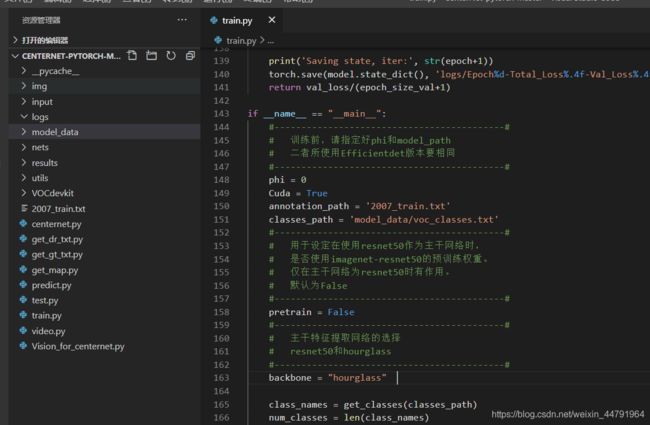
然后运行train.py就可以开始训练啦。
运行train.py即可开始训练。
![]()