teengamb数据集进行回归分析
回归分析
在 faraway 包中,包含一个 47 行 5 列的 teengamb 数据集(加载 faraway包后,可通过代码“head(teengamb)”查看数据的前 5 行,通过“?teengamb”查看每个变量的具体意义),该数据是研究关于青少年赌博情况的数据集。针对该数据集,请回答以下问题:
Sex:性别,0=男性,1=女性。
Status:基于父母职业的社会经济状况评分
Income:每周的收入,英镑
Verbal:正确定义的 12 各单词的口头评分
Gamle:每年赌博的开支,英镑。
(1)如果只考虑 sex、income、verbal 三个变量作为自变量,预测因变量 gamble
时,可以使用哪些回归模型进行预测?要求建立的回归模型数量不少于 3 个,
并对为什么要建立这样的回归模型进行解释;
先进行相关系数分析:
library(corrplot)
library(faraway)
library(ggcorrplot)
library(tidyr)
library(GGally)
data(teengamb)
head(teengamb)
teengamb<-teengamb
?teengamb
teen<-data.frame(teengamb$sex,teengamb$income,teengamb$gamble,teengamb$verbal)
voice_cor <- cor(teen)
corrplot.mixed(voice_cor,tl.col="black",tl.pos = "lt",
               tl.cex = 2,number.cex = 1)
结果如下:
> head(teengamb)
  sex status income verbal gamble
1   1     51   2.00      8    0.0
2   1     28   2.50      8    0.0
3   1     37   2.00      6    0.0
4   1     28   7.00      4    7.3
5   1     65   2.00      8   19.6
6   1     61   3.47      6    0.1
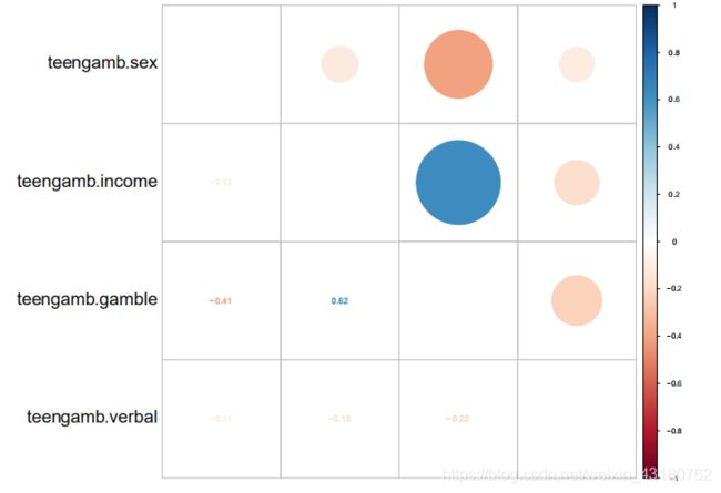
可发现,income 和 gamble 收入相关性达到 0.62,较强相关,gamble 与 sex 相关系数为-0.41,成一定相关性,说明与性别有关系。
再进行多元线性回归:
## 多元线型回归
lm1 <- lm(gamble~sex+income+verbal,data = teengamb)
summary(lm1)
结果如下:
> summary(lm1)

Call:
lm(formula = gamble ~ sex + income + verbal, data = teengamb)

Residuals:
    Min      1Q  Median      3Q     Max
-50.639 -11.765  -1.594   9.305  93.867

Coefficients:
            Estimate Std. Error t value Pr(>|t|)
(Intercept)  24.1390    14.7686   1.634   0.1095
sex         -22.9602     6.7706  -3.391   0.0015 **
income        4.8981     0.9551   5.128 6.64e-06 ***
verbal       -2.7468     1.8253  -1.505   0.1397
---
Signif. codes:  0 ‘***’ 0.001 ‘**’ 0.01 ‘*’ 0.05 ‘.’ 0.1 ‘ ’ 1

Residual standard error: 22.43 on 43 degrees of freedom
Multiple R-squared:  0.5263,	Adjusted R-squared:  0.4933
F-statistic: 15.93 on 3 and 43 DF,  p-value: 4.148e-07
经多元线性回归,系数检验发现,verbal 检验的 p 值为 0.1397>0.05,不显著,故可考虑剔除 verbal 做多元线性回归。
考虑剔除verbal :
#剔除verbal
lm2 <- lm(gamble~sex+income,data = teengamb)
summary(lm2)
library(broom)
## 可视化回归模型的图像
par(mfrow = c(2,2))
plot(lm2)
结果如下:
> summary(lm2)

Call:
lm(formula = gamble ~ sex + income, data = teengamb)

Residuals:
    Min      1Q  Median      3Q     Max
-49.757 -11.649   0.844   8.659 100.243

Coefficients:
            Estimate Std. Error t value Pr(>|t|)
(Intercept)    4.041      6.394   0.632  0.53070
sex          -21.634      6.809  -3.177  0.00272 **
income         5.172      0.951   5.438 2.24e-06 ***
---
Signif. codes:  0 ‘***’ 0.001 ‘**’ 0.01 ‘*’ 0.05 ‘.’ 0.1 ‘ ’ 1

Residual standard error: 22.75 on 44 degrees of freedom
Multiple R-squared:  0.5014,	Adjusted R-squared:  0.4787
F-statistic: 22.12 on 2 and 44 DF,  p-value: 2.243e-07
可发现,参数的检验 sex,income 都较为显著,而 Adjusted R-squared=0.4787
可得到回归方程:
gamble = 4.041 − 21.634 ∗ sex + 5.172 ∗ income

再进行逐步线性回归:
Enblm <- lm(gamble~sex+income+verbal,data = teengamb)
summary(Enblm)
## Coefficients: (1 not defined because of singularities)
## 因为奇异性问题,有一个变量没有计算系数
## 判断模型的多重共线性问题
kappa(Enblm,exact=TRUE) #exact=TRUE表示精确计算条件数;
alias(Enblm)
## 逐步回归
Enbstep <- step(Enblm,direction = "both")
summary(Enbstep)
## 判断模型的多重共线性问题
kappa(Enbstep,exact=TRUE)
vif(Enbstep)
结果如下:
> Enbstep <- step(Enblm,direction = "both")
Start:  AIC=296.21
gamble ~ sex + income + verbal

         Df Sum of Sq   RSS    AIC
<none>                21642 296.21
- verbal  1    1139.8 22781 296.63
- sex     1    5787.9 27429 305.35
- income  1   13236.1 34878 316.64

> summary(Enbstep)

Call:
lm(formula = gamble ~ sex + income + verbal, data = teengamb)

Residuals:
    Min      1Q  Median      3Q     Max
-50.639 -11.765  -1.594   9.305  93.867

Coefficients:
            Estimate Std. Error t value Pr(>|t|)
(Intercept)  24.1390    14.7686   1.634   0.1095
sex         -22.9602     6.7706  -3.391   0.0015 **
income        4.8981     0.9551   5.128 6.64e-06 ***
verbal       -2.7468     1.8253  -1.505   0.1397
---
Signif. codes:  0 ‘***’ 0.001 ‘**’ 0.01 ‘*’ 0.05 ‘.’ 0.1 ‘ ’ 1

Residual standard error: 22.43 on 43 degrees of freedom
Multiple R-squared:  0.5263,	Adjusted R-squared:  0.4933
F-statistic: 15.93 on 3 and 43 DF,  p-value: 4.148e-07

> kappa(Enbstep,exact=TRUE)
[1] 39.20124
> vif(Enbstep)
     sex   income   verbal
1.030968 1.051585 1.049578
可发现,不存在多重共线性,故结果将与多元线性回归一致。
(2)使用所有的变量预测因变量 gamble,并且使用 step()函数对模型进行逐步回归,分析逐步回归后的结果;
Enblm <- lm(gamble~sex+income+verbal+status,data = teengamb)
summary(Enblm)
## Coefficients: (1 not defined because of singularities)
## 因为奇异性问题,有一个变量没有计算系数
## 判断模型的多重共线性问题
kappa(Enblm,exact=TRUE) #exact=TRUE表示精确计算条件数;
alias(Enblm)
## 逐步回归
Enbstep <- step(Enblm,direction = "both")
summary(Enbstep)
## 判断模型的多重共线性问题
kappa(Enbstep,exact=TRUE)
vif(Enbstep)
结果如下:
#原始状态,未剔除变量
> summary(Enblm)

Call:
lm(formula = gamble ~ sex + income + verbal + status, data = teengamb)

Residuals:
    Min      1Q  Median      3Q     Max
-51.082 -11.320  -1.451   9.452  94.252

Coefficients:
             Estimate Std. Error t value Pr(>|t|)
(Intercept)  22.55565   17.19680   1.312   0.1968
sex         -22.11833    8.21111  -2.694   0.0101 *
income        4.96198    1.02539   4.839 1.79e-05 ***
verbal       -2.95949    2.17215  -1.362   0.1803
status        0.05223    0.28111   0.186   0.8535
---
Signif. codes:  0 ‘***’ 0.001 ‘**’ 0.01 ‘*’ 0.05 ‘.’ 0.1 ‘ ’ 1

Residual standard error: 22.69 on 42 degrees of freedom
Multiple R-squared:  0.5267,	Adjusted R-squared:  0.4816
F-statistic: 11.69 on 4 and 42 DF,  p-value: 1.815e-06

> kappa(Enblm,exact=TRUE) #exact=TRUE表示精确计算条件数;
[1] 263.8049
> alias(Enblm)
Model :
gamble ~ sex + income + verbal + status
#此时存在多重共线性,条件数为263,较大


#逐步回归后:
> Enbstep <- step(Enblm,direction = "both")
Start:  AIC=298.18
gamble ~ sex + income + verbal + status

         Df Sum of Sq   RSS    AIC
- status  1      17.8 21642 296.21
<none>                21624 298.18
- verbal  1     955.7 22580 298.21
- sex     1    3735.8 25360 303.67
- income  1   12056.2 33680 317.00

Step:  AIC=296.21
gamble ~ sex + income + verbal

         Df Sum of Sq   RSS    AIC
<none>                21642 296.21
- verbal  1    1139.8 22781 296.63
+ status  1      17.8 21624 298.18
- sex     1    5787.9 27429 305.35
- income  1   13236.1 34878 316.64
> summary(Enbstep)

Call:
lm(formula = gamble ~ sex + income + verbal, data = teengamb)

Residuals:
    Min      1Q  Median      3Q     Max
-50.639 -11.765  -1.594   9.305  93.867

Coefficients:
            Estimate Std. Error t value Pr(>|t|)
(Intercept)  24.1390    14.7686   1.634   0.1095
sex         -22.9602     6.7706  -3.391   0.0015 **
income        4.8981     0.9551   5.128 6.64e-06 ***
verbal       -2.7468     1.8253  -1.505   0.1397
---
Signif. codes:  0 ‘***’ 0.001 ‘**’ 0.01 ‘*’ 0.05 ‘.’ 0.1 ‘ ’ 1

Residual standard error: 22.43 on 43 degrees of freedom
Multiple R-squared:  0.5263,	Adjusted R-squared:  0.4933
F-statistic: 15.93 on 3 and 43 DF,  p-value: 4.148e-07

#R方为0.4933,P值<0.05,模型检验通过。

> kappa(Enbstep,exact=TRUE)
[1] 39.20124
> vif(Enbstep)
     sex   income   verbal
1.030968 1.051585 1.049578
逐步回归之后,回归模型的条件数变为 39.20124,此时剔除了 status 变量。
(3)如果以性别为因变量,能够根据其他的几个数据特征准确地预测出性别吗?如果可以,那么预测的准确率是多少?如果不可以,请说明为什么?
利用逻辑斯特回归预测:
library(caret)
library(Metrics)
library(dplyr)

voicelm <- glm(sex~.,data = teengamb,family = "binomial")#利用逻辑斯特回归预测
summary(voicelm)
label<-predict(voicelm,teengamb[,2:5],type = "response")
label <- as.factor(ifelse(label > 0.5,1,0))#将数据规范为0,1
table(teengamb$sex,label)
sprintf("逻辑回归模型的精度为:%f",accuracy(teengamb$sex,label))
结果如下:
> summary(voicelm)

Call:
glm(formula = sex ~ ., family = "binomial", data = teengamb)

Deviance Residuals:
     Min        1Q    Median        3Q       Max
-1.50499  -0.57882  -0.09388   0.59949   2.58612

Coefficients:
            Estimate Std. Error z value Pr(>|z|)
(Intercept)  3.63905    1.90352   1.912   0.0559 .
status      -0.10108    0.04033  -2.507   0.0122 *
income       0.10653    0.18900   0.564   0.5730
verbal       0.13822    0.25711   0.538   0.5909
gamble      -0.08651    0.04247  -2.037   0.0417 *
---
Signif. codes:  0 ‘***’ 0.001 ‘**’ 0.01 ‘*’ 0.05 ‘.’ 0.1 ‘ ’ 1

(Dispersion parameter for binomial family taken to be 1)

    Null deviance: 63.422  on 46  degrees of freedom
Residual deviance: 36.140  on 42  degrees of freedom
AIC: 46.14

Number of Fisher Scoring iterations: 7

> table(teengamb$sex,label)
   label
     0  1
  0 23  5
  1  4 15
> sprintf("逻辑回归模型的精度为:%f",accuracy(teengamb$sex,label))
[1] "逻辑回归模型的精度为:0.808511"
精度为80%,较低,可尝试使用深度学习方法和支持向量机等机器学习方法。详细可参加另一篇文章《对于teengamb数据集进行神经网络分类》