TensorFlow-Keras 15.Wide & Deep

一.引言

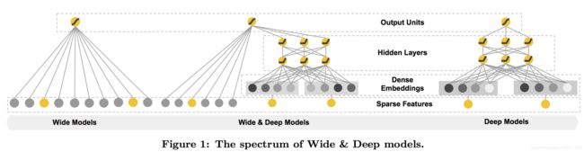
Wide & Deep 模型的提出不仅结合了 Wide(线性模型)的记忆能力，同时结合了Deep(深度)的泛化能力，其在2016年由谷歌提出。记忆能力可以理解为模型直接学习历史数据的共现频率能力，结构简单也造成了原始数据很容易影响推算结果。泛化能力可以被理解为模型传递特征的相关性，以及挖掘稀疏甚至从未出现过的稀有特征的能力，矩阵分解能够优于协同过滤，就是因为加入了隐向量，丰富了稀疏特征的表示，Deep侧通过特征的多次自动组合，可以深度挖掘数据潜在的模式，即使是很稀疏的输入，也可以获取较为平滑的推算结果。下面就是基础的Wide & Deep模型架构，可以理解为 LR + DNN 的组合推荐，通过同时训练两个模型得到最终的预测结果。

 

二.BaseLine Deep

前边我们说到，评价一个模型需要制定一个基准，Wide & Deep 的基准就定为一个单独的纯 Deep 模型。手写数字识别前面的博客中提到过，这里我们使用单512隐层，下面看看准确率如何。

    (train_images, train_labels),(test_images,test_labels) = mnist.load_data()
    print("训练集维度: " ,train_images.shape)

    network = models.Sequential()
    network.add(layers.Dense(512, activation='relu', input_shape=(28 * 28,)))
    network.add(layers.Dense(10, activation='softmax'))

    network.compile(optimizer='rmsprop',
                    loss='categorical_crossentropy',
                    metrics=['accuracy'])

    train_images = train_images.reshape((60000, 28 * 28))
    train_images = train_images.astype('float32') / 255

    test_images = test_images.reshape((10000, 28 * 28))
    test_images = test_images.astype('float32') / 255

    print(train_labels[0])
    print(train_labels.shape)
    train_labels = to_categorical(train_labels)
    print(train_labels[0])
    print(train_labels.shape)

    test_labels = to_categorical(test_labels)

    network.fit(train_images, train_labels, epochs=5, batch_size=128)
    test_loss, test_acc = network.evaluate(test_images, test_labels)
    print("test_acc", test_acc, " test_loss", test_loss)

训练结果:

......

Epoch 4/5
469/469 [==============================] - 1s 2ms/step - loss: 0.0485 - accuracy: 0.9857
Epoch 5/5
469/469 [==============================] - 1s 1ms/step - loss: 0.0345 - accuracy: 0.9899

验证结果:

313/313 [==============================] - 0s 281us/step - loss: 0.0660 - accuracy: 0.9808

Epoch = 5，batch_size = 128 的情况下 训练 Loss ，训练 Acc，验证 Loss，验证 Acc 如上 ⬆️ 

 

三.Wide & Deep 简易版实现

这里选择机器学习非常常见的mnist手写数字识别测试样例测试，原始数据是 Sampes x 784(28 * 28) 的图片像素数组，我们通过 LR + DNN 实现其分类效果。这个是简单一点的实现，这里可以理解为将原始数据打平，无差别的将 Hidden 层的激活与原始数据 concat,最后接一个Dense输出结果。

 

    (train_images, train_labels),(test_images,test_labels) = mnist.load_data()

    train_images = train_images.reshape((60000, 28 * 28))
    train_images = train_images.astype('float32') / 255

    test_images = test_images.reshape((10000, 28 * 28))
    test_images = test_images.astype('float32') / 255

    input = layers.Input(shape=train_images.shape[1:])
    hidden1 = layers.Dense(512, activation="relu")(input)

    concat = layers.concatenate([input, hidden1],axis=-1)
    output = layers.Dense(10, activation='softmax')(concat)
    model = Model(inputs=[input], outputs=[output])
    model.compile(optimizer='rmsprop',
                    loss='categorical_crossentropy',
                    metrics=['accuracy'])
    model.summary()
    train_labels = to_categorical(train_labels)
    test_labels = to_categorical(test_labels)

    model.fit(train_images, train_labels, epochs=5, batch_size=128)
    test_loss, test_acc = model.evaluate(test_images, test_labels)
    print("test_acc", test_acc, " test_loss", test_loss)

 训练结果:

......

Epoch 4/5
469/469 [==============================] - 1s 2ms/step - loss: 0.0517 - accuracy: 0.9842
Epoch 5/5
469/469 [==============================] - 1s 2ms/step - loss: 0.0380 - accuracy: 0.9891

验证结果:

313/313 [==============================] - 0s 296us/step - loss: 0.0752 - accuracy: 0.9771

这里只用了1个隐层 Hidden1，并未按照上图架构是因为想和 baseline作对比。可以看到效果略差于 BaseLine 的纯 Deep 版本，在手写数字图像识别场景下加入 LR 可能对于推荐结果没有过大的影响，如果是在推荐场景下，Wide & Deep 应该会相比 Deep 有更好的表征，因为手写数字识别数据不涉及稀疏输入，它的数据都是完整的像素数组，其次手写数字识别的像素点之间存在一定程度的共线性（相邻的像素较为相似），因此不加区分加入到 LR 模型中会造成一定影响，这里如果把 concat 时的原始 input 切换为抽样或者局部处理的数据，可能会带来更好的效果，这里实现一个简单的将 Step 内的数据求和并输出的自定义层，有兴趣的小伙伴可以自己修改并应用到上述 demo :

class MyLayer(Layer):

    def bulid(self, input_shape):
        # create a trainable weight variable for this layer
        self.kernel = self.add_weight(name='kernel',
                                      shape=(input_shape[1], self.output_dim),
                                      initializer='uniform',
                                      trainable=True)
        super(MyLayer, self).build(input_shape)  # Be sure to call this at the end

    def call(self, inputs, step=3, **kwargs):
        result = []
        for i in range(0, inputs.shape[1], step):
            result.append(K.sum(inputs[i:i + step]))
        return result

    def compute_output_shape(self, input_shape):
        return (input_shape[0], self.output_dim)

    arr = list(range(0,100))
    layer = MyLayer()
    result = layer(arr, output_dim=len(arr)/3)
    print(np.asarray(result))

结果：

原始数组为 0,1,2,3... 每三个数据求和得到一个结果 ⬇️

[  3  12  21  30  39  48  57  66  75  84  93 102 111 120 129 138 147 156
 165 174 183 192 201 210 219 228 237 246 255 264 273 282 291  99]

 

四.Wide & Deep 进阶版实现

上面我们提到 Wide & Deep 更多用于推荐场景，接下来我们使用稍微复杂的 Deep 模型实现 Wide & Deep，数据还是使用 mnist 手写数字识别数据，只不过这里我们把它当模拟为推荐系统中的连续数据，除此之外我们还会加入额外的人工数据，因此只关注模型实现，不关注模型最终预测结果。

user-item 推荐中，往往有稀疏的类别特征，如果 one-hot 得到稀疏向量送进 Deep 模型或者 LR 模型都不能很好地表征特征，且得到的模型泛化能力不足，基于这个原因 Wide & Deep 提出将离散特征放入 LR 学习，离散的类别特征通过引入 Embedding 层泛化其表征，随后接入隐层，所以架构就是连续特征 ➡️  放入 Wide 部分，离散类别特征 ➡️  放入 Deep 模型，并引入 Embedding。

1.Wide Part

wide 部分与简易版相同，直接使用 None x 784 的数据作为推荐模型 LR 的离散数据

    (train_images, train_labels),(test_images,test_labels) = mnist.load_data()

    # wide部分
    train_images = train_images.reshape((60000, 28 * 28))
    train_images = train_images.astype('float32') / 255

    test_images = test_images.reshape((10000, 28 * 28))
    test_images = test_images.astype('float32') / 255

    wideInput = layers.Input(shape=train_images.shape[1:], name='wide')

 

2.Deep Part

上面 Deep 将连续数据打平直接连接了 Dense 层，这里我们基于假设的推荐场景存在两个类别特征A、B，每个类别都有100中可能的情况，这里用 categoryA 与 categoryB 随机模拟该稀疏特征，随后将其拼接为 NumSamples x 2 的原始数据，随后通过 Embedding 层将原始的类别特征嵌入到 128 维的 Embedding中再连入 Dense。

    # Deep部分
    num_samples = 60000
    categoryA = np.random.randint(0, 100, (num_samples, 1))
    categoryB = np.random.randint(100, 200, (num_samples, 1))
    concat = np.concatenate([categoryA, categoryB], axis=-1)

    deepInput = layers.Input(shape=2, name='deep')
    embedding = layers.Embedding(200, 128, input_length=2)(deepInput)
    hidden = layers.Dense(512, activation="relu")(embedding)
    flatten = layers.Flatten()(hidden)

 

3.Concat & Train

通过 layers.concatenate 实现 LR + Deep 激活的拼接，最终通过 softmax 预测最终结果，由于 Category A,B 是随机人工引入的，因此训练 Loss, Acc 不做参考。

    # 合并
    concatWideAndDeep = layers.concatenate([wideInput, flatten], axis=-1)

    # 模型编译
    output = layers.Dense(10, activation='softmax')(concatWideAndDeep)
    model = Model(inputs=[wideInput, deepInput], outputs=[output])
    model.compile(optimizer='rmsprop',
                    loss='categorical_crossentropy',
                    metrics=['accuracy'])
    model.summary()

    train_labels = to_categorical(train_labels)
    test_labels = to_categorical(test_labels)

    print(train_images.shape, concat.shape)
    model.fit({'wide': train_images, 'deep': concat}, train_labels, epochs=5, batch_size=128)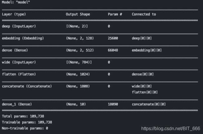

......

Epoch 4/5
469/469 [==============================] - 1s 1ms/step - loss: 0.2777 - accuracy: 0.9211
Epoch 5/5
469/469 [==============================] - 1s 1ms/step - loss: 0.2750 - accuracy: 0.9228

 

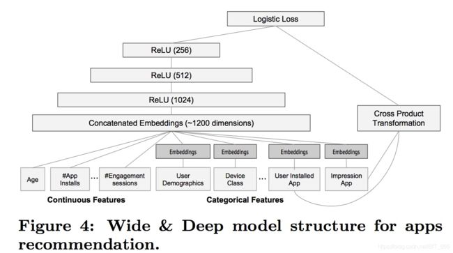
五.Wide & Deep 进阶版 - 推荐引擎

参考上述模拟推荐场景，这里连续型特征 + 离散特征的 one-hot : Age，App Installs，Engagement 直接接入 Concat Dense 层，除此之外类别的离散特征 : User Demographics (用户统计)，Device(设备) 等分别通过 Embedding 向量化后 concat 进同一 Dense 层，上述是 Wide & Deep 的实现，在此基础上增加了三层 Relu 激活且对 App 的离散特征得到的 Embedding 进行了手动交叉，类似于 FM 的隐向量相乘，最终将全部数据送到 LR，相比上面实现的 Demo 版 Wide & Deep 加入了更多的隐层，更多的  Embedding 泛化以及人工自定义的交叉，所以模型的表达能力更强，由于没有足够数据这里就不展示代码了，有兴趣的同学可以自己实现~