python查看网络的特征图,并计算特征图的直方图,并计算香农熵。
查看特征图的原理
在网络的每一层输出中,都会输出一个[b,c,h,w]维度的数据,b是batch的大小,c是通道数,h,w是高和宽。
比如某一层的特征图是32x64x112x122,即batch大小为32,通道数为64,大小为112x112的图像。
我们读取到这个数据32x64x112x122之后,将其batch维度压缩掉,然后在转换成为图像的PIL格式,即112x112x64.
这也就意味着我们有64个112x112大小的图像,我们只需要读取每个通道的图像就可以看到特征图。
1.获取输出
在pytorch构建网络时,会有一个forward函数,在里面添加我们想要看到的特征层数据:
    def forward(self, x):
        outputs=[]
        x1=self.rnn1(x)
        outputs.append(x1)
        x2=self.rnn(x1)
        outputs.append(x2)
        x5 = self.features(x2)
        outputs.append(x5)
        x5= torch.flatten(x5, start_dim=1)
        x5= self.classifier(x5)
        return x5,outputs
即我想要看到是第一个卷积的输出,第二个卷积的输出,以及最后一个卷积的输出,这三个特征层的输出就是我们获取到的[b,c,h,w]数据。
2.载入模型,来源:B站博主
import torch
from alexnet_model import AlexNet
from resnet_model import resnet34
import matplotlib.pyplot as plt
import numpy as np
from PIL import Image
from torchvision import transforms

data_transform = transforms.Compose(
    [transforms.Resize((224, 224)),
     transforms.ToTensor(),
     transforms.Normalize((0.5, 0.5, 0.5), (0.5, 0.5, 0.5))])

# data_transform = transforms.Compose(
#     [transforms.Resize(256),
#      transforms.CenterCrop(224),
#      transforms.ToTensor(),
#      transforms.Normalize([0.485, 0.456, 0.406], [0.229, 0.224, 0.225])])

# create model
model = AlexNet(num_classes=5)
# model = resnet34(num_classes=5)
# load model weights
model_weight_path = "./AlexNet.pth"  # "./resNet34.pth"
model.load_state_dict(torch.load(model_weight_path))
print(model)

# load image
img = Image.open("../tulip.jpg")
# [N, C, H, W]
img = data_transform(img)
# expand batch dimension
img = torch.unsqueeze(img, dim=0)

# forward
out_put = model(img)
for feature_map in out_put:
    # [N, C, H, W] -> [C, H, W]
    im = np.squeeze(feature_map.detach().numpy())
    # [C, H, W] -> [H, W, C]
    im = np.transpose(im, [1, 2, 0])

    # show top 12 feature maps
    plt.figure()
    for i in range(12):
        ax = plt.subplot(3, 4, i+1)
        # [H, W, C]
        plt.imshow(im[:, :, i], cmap='gray')
    plt.show()
按照我们的需要对其进行修改,并查看结果:
# create model
model_name = "vgg16"
model=vgg(model_name=model_name, num_classes=102, init_weights=False)
# model = resnet34(num_classes=5)
# load model weights
model_weight_path = "./vgg16_12_BN_best.pth"  # "./resNet34.pth"
model.load_state_dict(torch.load(model_weight_path))
print(model)

# load image
img = Image.open("./car0.jpg")
# [N, C, H, W]
img = data_transform(img)
# expand batch dimension
img = torch.unsqueeze(img, dim=0)

# forward
_,out_put =model(img)
for feature_map in out_put:
    # [N, C, H, W] -> [C, H, W]
    im = np.squeeze(feature_map.detach().numpy())
    # [C, H, W] -> [H, W, C]
    im = np.transpose(im, [1, 2, 0])
    # show top 12 feature maps
    plt.figure()
    for i in range(12):
        ax = plt.subplot(3, 4, i+1)
        # [H, W, C]
        plt.imshow(im[:, :, i], cmap='gray')
    plt.show()
查看的结果是每个输出的前12通道的图像,结果如下:

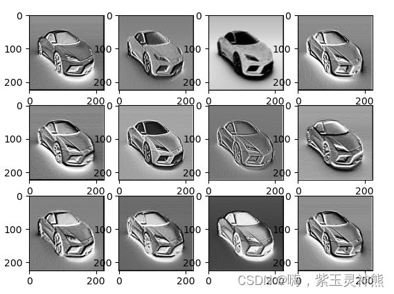

卷积卷到最后就是一些抽象的东西,网络根据最后一个卷积的输出,进行分类判别。
计算直方图和香农熵
计算直方图时,我是将一个输出融合成为了一张图像,比如32x64x112x122的输出,最后变成了1x122x122,实现这一步的操作是用了一个1x1的卷积,并且将其卷积的权重全部赋值为1.
将输出融合成一张图像:
_,out_put =model(img)
for feature_map in out_put:
# [N, C, H, W] -> [C, H, W]
conv4 = torch.nn.Conv2d(feature_map.shape[1], 1, 1, 1)
ones = torch.Tensor(np.ones([1, feature_map.shape[1], 1, 1]))
conv4.weight = torch.nn.Parameter(ones)
feature_map=conv4(feature_map)
print(feature_map.shape)
im = np.squeeze(feature_map.detach().numpy())
plt.imshow(im)
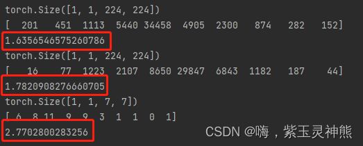
plt.show()计算直方图和香农熵
_,out_put =model(img)
for feature_map in out_put:
    # [N, C, H, W] -> [C, H, W]
    conv4 = torch.nn.Conv2d(feature_map.shape[1], 1, 1, 1)
    ones = torch.Tensor(np.ones([1, feature_map.shape[1], 1, 1]))
    conv4.weight = torch.nn.Parameter(ones)
    feature_map=conv4(feature_map)
    print(feature_map.shape)
    im = np.squeeze(feature_map.detach().numpy())
    plt.imshow(im)
    plt.show()
    # img.ravel() 将图像转成一维数组,这里没有中括号。
    hist, bins = np.histogram(im.ravel())
    plt.hist(im)
    plt.show()
    A = np.array(hist)
    print(A)
    pa = A / A.sum()
    shanno = -np.sum(pa * np.log2(pa+0.000000001))
    print(shanno)
结果如下:


香农熵的计算公式为:
H(u)=E[-log(pi)] = sum(-(pi*log(2)pi))
计算的结果为: