pytorch贝叶斯网络
Hyperparameters are the parameters in models that determine model architecture, learning speed and scope, and regularization.
超参数是确定模型架构,学习速度和范围以及正则化的模型中的参数。
The search for optimal hyperparameters requires some expertise and patience, and you’ll often find people using exhausting methods like grid search and random search to find the hyperparameters that work best for their problem.
寻找最佳超参数需要一定的专业知识和耐心,并且您经常会发现一些人使用诸如网格搜索和随机搜索之类的精疲力尽的方法来找到最适合其问题的超参数。
快速教程 (A quick tutorial)
I’m going to show you how to implement Bayesian optimization to automatically find the optimal hyperparameter set for your neural network in PyTorch using Ax.
我将向您展示如何实现贝叶斯优化,以使用Ax在PyTorch中自动为您的神经网络找到最佳超参数集。
We’ll be building a simple CIFAR-10 classifier using transfer learning. Most of this code is from the official PyTorch beginner tutorial for a CIFAR-10 classifier.
我们将使用迁移学习构建一个简单的CIFAR-10分类器。 大部分代码来自CIFAR-10分类器的官方PyTorch初学者教程。
I won’t be going into the details of Bayesian optimization, but you can study the algorithm on the Ax website, read the original paper or the 2012 paper on its practical use.
我不会介绍贝叶斯优化的细节,但是您可以在Ax网站上研究该算法,阅读原始论文或2012年论文的实际用法。
首先,通常 (Firstly, the usual)
Install Ax using:
使用以下方法安装Ax:
pip install ax-platformImport all the necessary libraries:
导入所有必需的库:
import matplotlib.pyplot as plt
import numpy as np
import torch
import torchvision
import torchvision.transforms as transforms
import torch.optim as optim
import torch.nn as nn
import torch.nn.functional as F


from ax.plot.contour import plot_contour
from ax.plot.trace import optimization_trace_single_method
from ax.service.managed_loop import optimize
from ax.utils.notebook.plotting import render
from ax.utils.tutorials.cnn_utils import train, evaluate


device = torch.device("cuda:0" if torch.cuda.is_available() else "cpu")
Download the datasets and construct the data loaders (I would advise adjusting the training batch size to 32 or 64 later):
下载数据集并构造数据加载器(我建议稍后将训练批处理大小调整为32或64):
device = torch.device("cuda:0" if torch.cuda.is_available() else "cpu")


# Assuming that we are on a CUDA machine, this should print a CUDA device:


print(device)


transform = transforms.Compose(
    [transforms.ToTensor(),
     transforms.Normalize((0.5, 0.5, 0.5), (0.5, 0.5, 0.5))])


trainset = torchvision.datasets.CIFAR10(root='./data', train=True,
                                        download=True, transform=transform)
trainloader = torch.utils.data.DataLoader(trainset, batch_size=4,
                                          shuffle=True, num_workers=2)


testset = torchvision.datasets.CIFAR10(root='./data', train=False,
                                       download=True, transform=transform)
testloader = torch.utils.data.DataLoader(testset, batch_size=4,
                                         shuffle=False, num_workers=2)


classes = ('plane', 'car', 'bird', 'cat',
           'deer', 'dog', 'frog', 'horse', 'ship', 'truck')
Let’s take a look at the CIFAR-10 dataset by creating some helper functions:
让我们通过创建一些辅助函数来看看CIFAR-10数据集:
def imshow(img):
    img = img / 2 + 0.5     # unnormalize
    npimg = img.numpy()
    plt.imshow(np.transpose(npimg, (1, 2, 0)))
    plt.show()


# get some random training images
dataiter = iter(trainloader)
images, labels = dataiter.next()


# show images
imshow(torchvision.utils.make_grid(images))
# print labels
print(' '.join('%5s' % classes[labels[j]] for j in range(4)))培训和评估职能(Training and evaluation functions)
Ax requires a function that returns a trained model, and another that evaluates a model and returns a performance metric like accuracy or F1 score. We’re only building the training function here and using Ax’s ownevaluate tutorial function to test our model performance, which returns accuracy. You can check out ther API to model your own evaluation function after theirs, if you’d like.
Axe需要一个函数来返回经过训练的模型,而另一个函数则需要对模型进行评估并返回诸如准确性或F1分数之类的性能指标。 我们仅在此处构建训练功能,并使用Ax自己的evaluate教程功能来测试我们的模型性能,这将返回准确性。 如果需要,您可以签出API来对自己的评估函数进行建模。
def net_train(net, train_loader, parameters, dtype, device):
  net.to(dtype=dtype, device=device)


  # Define loss and optimizer
  criterion = nn.CrossEntropyLoss()
  optimizer = optim.SGD(net.parameters(), # or any optimizer you prefer
                        lr=parameters.get("lr", 0.001), # 0.001 is used if no lr is specified
                        momentum=parameters.get("momentum", 0.9)
  )


  scheduler = optim.lr_scheduler.StepLR(
      optimizer,
      step_size=int(parameters.get("step_size", 30)),
      gamma=parameters.get("gamma", 1.0),  # default is no learning rate decay
  )


  num_epochs = parameters.get("num_epochs", 3) # Play around with epoch number
  # Train Network
  for _ in range(num_epochs):
      for inputs, labels in train_loader:
          # move data to proper dtype and device
          inputs = inputs.to(dtype=dtype, device=device)
          labels = labels.to(device=device)


          # zero the parameter gradients
          optimizer.zero_grad()


          # forward + backward + optimize
          outputs = net(inputs)
          loss = criterion(outputs, labels)
          loss.backward()
          optimizer.step()
          scheduler.step()
  return net
Next, we’re writing an init_net() function that initializes the model and returns the network ready-to-train. There are many opportunities for hyperparameter tuning here. You’ll notice the parameterization argument, which is a dictionary containing the hyperparameters.
接下来,我们正在编写一个init_net()函数,该函数初始化模型并返回准备训练的网络。 这里有许多进行超参数调整的机会。 您会注意到parameterization参数,它是包含超parameterization的字典。
def init_net(parameterization):


    model = torchvision.models.resnet50(pretrained=True) #pretrained ResNet50


    # The depth of unfreezing is also a hyperparameter
    for param in model.parameters():
        param.requires_grad = False # Freeze feature extractor

    Hs = 512 # Hidden layer size; you can optimize this as well

    model.fc = nn.Sequential(nn.Linear(2048, Hs), # attach trainable classifier
                                 nn.ReLU(),
                                 nn.Dropout(0.2),
                                 nn.Linear(Hs, 10),
                                 nn.LogSoftmax(dim=1))
    return model # return untrained model
Lastly, we need a train_evaluate() function that the Bayesian optimizer calls on every run. The optimizer generates a new set of hyperparameters in parameterization, passes it to this function, and then analyzes the returned evaluation results.
最后,我们需要一个train_evaluate()函数,该函数在每次运行时都会被贝叶斯优化器调用。 优化器在parameterization化中生成一组新的超parameterization ,将其传递给此函数,然后分析返回的评估结果。
def train_evaluate(parameterization):


    # constructing a new training data loader allows us to tune the batch size
    train_loader = torch.utils.data.DataLoader(trainset,
                                batch_size=parameterization.get("batchsize", 32),
                                shuffle=True,
                                num_workers=0,
                                pin_memory=True)

    # Get neural net
    untrained_net = init_net(parameterization)

    # train
    trained_net = net_train(net=untrained_net, train_loader=train_loader,
                            parameters=parameterization, dtype=dtype, device=device)

    # return the accuracy of the model as it was trained in this run
    return evaluate(
        net=trained_net,
        data_loader=testloader,
        dtype=dtype,
        device=device,
)优化!(Optimize!)
Now, just specify the hyperparameters you want to sweep across and pass that to Ax’s optimize() function:
现在,只需指定要扫描的超参数并将其传递给Ax的optimize()函数即可:
#torch.cuda.set_device(0) #this is sometimes necessary for me
dtype = torch.float
device = torch.device('cuda' if torch.cuda.is_available() else 'cpu')


best_parameters, values, experiment, model = optimize(
    parameters=[
        {"name": "lr", "type": "range", "bounds": [1e-6, 0.4], "log_scale": True},
        {"name": "batchsize", "type": "range", "bounds": [16, 128]},
        {"name": "momentum", "type": "range", "bounds": [0.0, 1.0]},
        #{"name": "max_epoch", "type": "range", "bounds": [1, 30]},
        #{"name": "stepsize", "type": "range", "bounds": [20, 40]},
    ],

    evaluation_function=train_evaluate,
    objective_name='accuracy',
)


print(best_parameters)
means, covariances = values
print(means)
print(covariances)
That sure took a while, but it’s nothing compared to doing a naive grid search for all 3 hyperparameters. Let’s take a look at the results:
确实花了一段时间,但与对所有3个超参数进行朴素的网格搜索相比,这没什么。 让我们看一下结果:
results[INFO 09-23 09:30:44] ax.modelbridge.dispatch_utils: Using Bayesian Optimization generation strategy: GenerationStrategy(name='Sobol+GPEI', steps=[Sobol for 5 arms, GPEI for subsequent arms], generated 0 arm(s) so far). Iterations after 5 will take longer to generate due to model-fitting.
[INFO 09-23 09:30:44] ax.service.managed_loop: Started full optimization with 20 steps.
[INFO 09-23 09:30:44] ax.service.managed_loop: Running optimization trial 1...
[INFO 09-23 09:31:55] ax.service.managed_loop: Running optimization trial 2...
[INFO 09-23 09:32:56] ax.service.managed_loop: Running optimization trial 3......[INFO 09-23 09:52:19] ax.service.managed_loop: Running optimization trial 18...
[INFO 09-23 09:53:20] ax.service.managed_loop: Running optimization trial 19...
[INFO 09-23 09:54:23] ax.service.managed_loop: Running optimization trial 20...{'lr': 0.000237872310800664, 'batchsize': 117, 'momentum':
{'accuracy': 0.4912998109307719}
{'accuracy': {'accuracy': 2.2924975426156455e-09}}
It seems our optimal learning rate is 2.37e-4 when comined with a momentum of 0.99 and a batch size of 117. That’s pretty nice. The 49.1% accuracy you see here is not the final accuracy of the model, so don’t worry!
似乎我们的最佳学习率是2.37e-4 ,而其动量为0.99且批量大小为117 。 很好您在此处看到的49.1%的精度不是模型的最终精度,所以请放心!
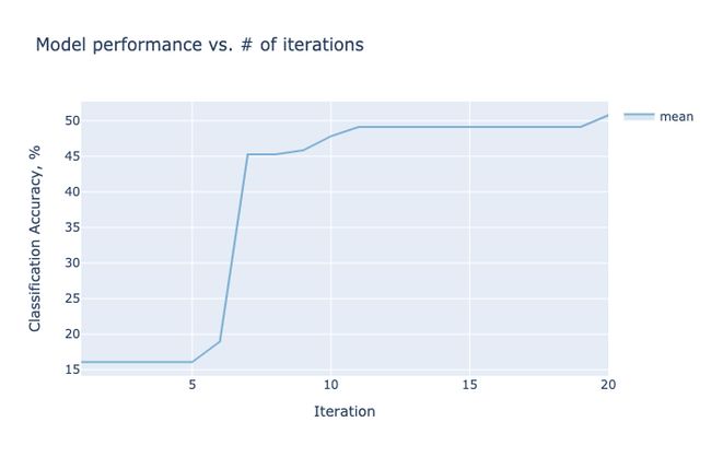
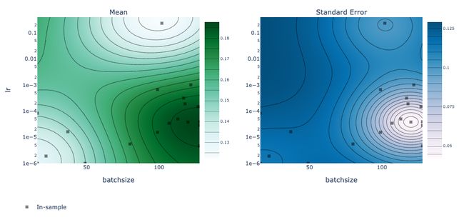
We can go even further and render some plots that show the accuracy per epoch (which improved as the parameterization improved), and the estimated accuracy by the optimizer as a function of two hyperparameters using a contour plot. The experiment variable is of type Experiment and you should definitely check out the docs to see all the methods it has to offer.
我们可以走得更远,绘制一些图,这些图显示每个时期的精度(随着参数化的改进而提高),以及优化器根据等高线图得出的两个超参数的函数所估计的精度。 该experiment变量的类型的Experiment ,你一定要检查出的文档看到所有它提供的方法。
best_objectives = np.array([[trial.objective_mean*100 for trial in experiment.trials.values()]])


best_objective_plot = optimization_trace_single_method(
    y=np.maximum.accumulate(best_objectives, axis=1),
    title="Model performance vs. # of iterations",
    ylabel="Classification Accuracy, %",
)
render(best_objective_plot)


render(plot_contour(model=model, param_x='batchsize', param_y='lr', metric_name='accuracy'))
The rendered plots are easy to understand and interactive. The black squares in the contour plots show the coordinates that have actually been sampled.
渲染的图易于理解和交互。 等高线图中的黑色正方形表示实际采样的坐标。
Lastly, you can fetch the parameter set (something Ax calls an “arm”) that has the best mean accuracy by simply running the script below:
最后,您可以通过简单地运行以下脚本来获取具有最高平均精度的参数集(Ax称其为“手臂”):
data = experiment.fetch_data()
df = data.df
best_arm_name = df.arm_name[df['mean'] == df['mean'].max()].values[0]
best_arm = experiment.arms_by_name[best_arm_name]
best_arm
Arm(name=’19_0', parameters={‘lr’: 0.00023787231080066353, ‘batchsize’: 117, ‘momentum’: 0.9914986635285268})Don’t be afraid to tune anything you wish, like hidden layer number and size, dropout, activation functions, depth of unfreezing, etc.
不要害怕调整任何您想要的东西,例如隐藏的层数和大小,退出,激活功能,解冻深度等。
Happy optimizing!
优化愉快!
翻译自: https://towardsdatascience.com/quick-tutorial-using-bayesian-optimization-to-tune-your-hyperparameters-in-pytorch-e9f74fc133c2
pytorch贝叶斯网络