【课程笔记】CS224N斯坦福自然语言处理

Course Homepage: http://web.stanford.edu/class/cs224n/

Lecture one

2021.2.25

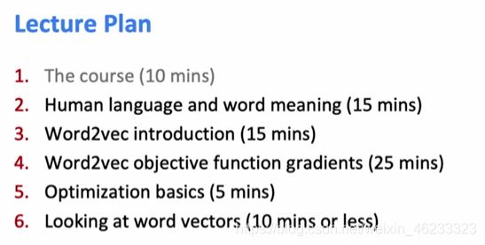
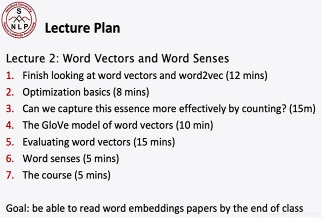
Plan of lecture one

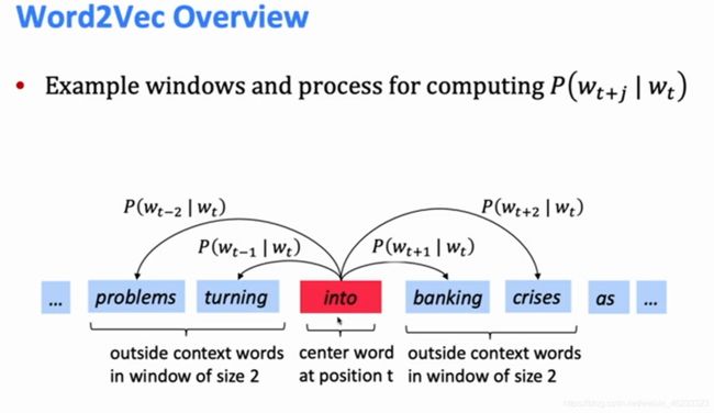
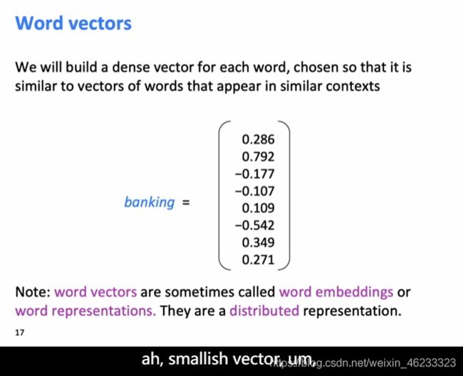
Distributed representation of word vector

A word’s meaning is given by the words that frequentlt appear closed-by.

“You should know a word by the company it keeps.”——J. R. Firth

Loss function:

Finally:

Before is trainning method, then this is prediction method:

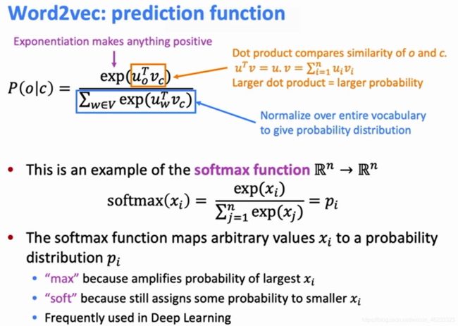
Use vectors’ dot multiply to calculate the simularity.
Now we need to calculate partial:

numerator is easy, look into denominator:
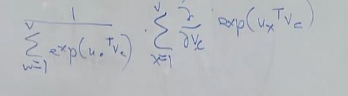
Use the chain rule:

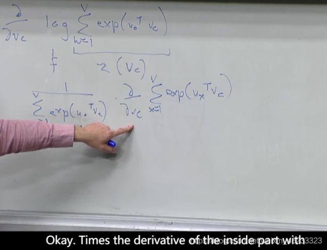
Then move the derivative inside the sum:

Use the chain rule again:

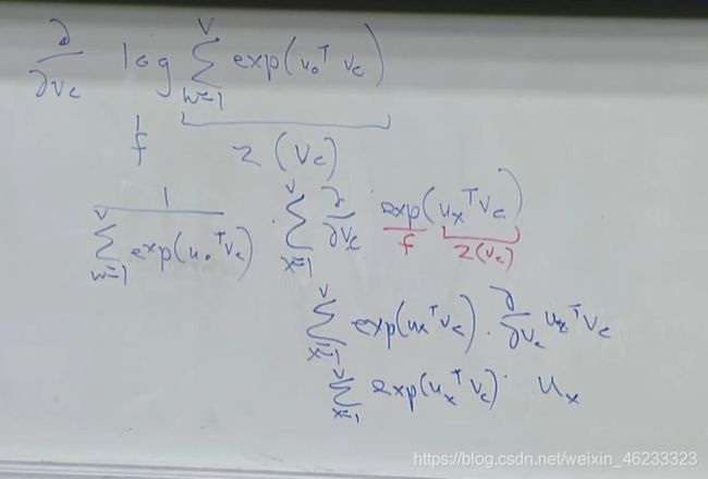
Finally:

Write it into a simple form:

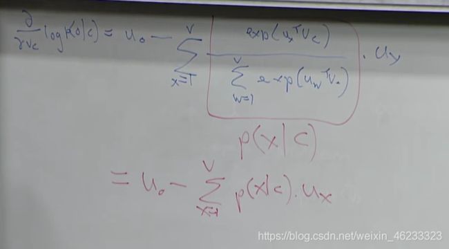
It means it takes the “difference” between the expected context word and the actual context word that showed up.

This difference give us the slope as to whcih direction we should be walking changing the words.
Exercise one
Solution of Exercise one

Lecture Two

More detail of word-embedding

Tricks

• SGD is faster, and can bring in some noise, which is equal to normalize the function.
• Objective function is nonconvex, so it is very important to choose a good starting point.
• ${\nabla }_{\theta }{J}_t(\theta )$ is very sparse! (Because only words in the window can be updated) So sometimes we use hashes or only update concerned rows in the matrix. Or we use Negative sampling transfer trhe probelm into binary classification.
  

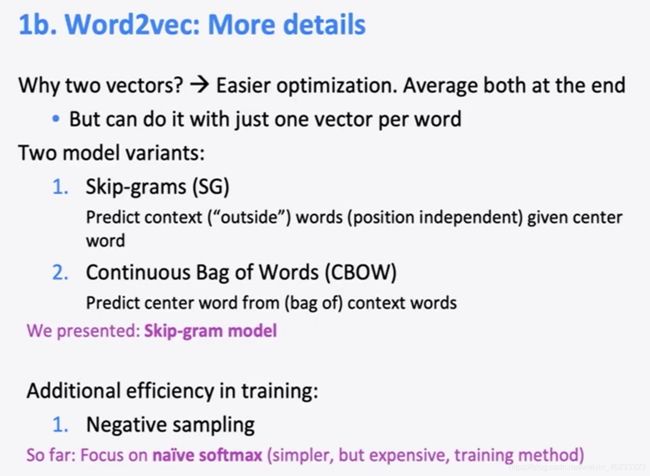
The idea of SG and CBOW is:

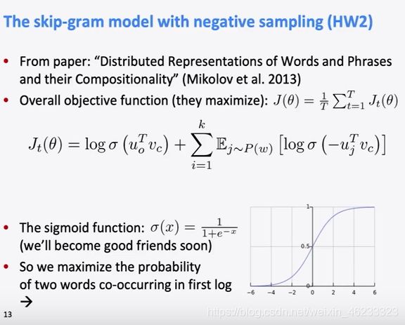
Negative Sampling: Train binary logistic regressions for a true pair(center word and word in its context window) versus a couple of noise pairs(the center word paired with a random word)

Here, The capital Z is often used as a normalization term:

So this is saying if you want the probability distribution of words, is you work out this three quaters power of the count of the word for every word in the vocabulary and then these numbers you just sum them up over the vocabulary and it’ll be sum total andf we’re dividing by that. So we get a probability distribution.

(Notes: In this class, Z means teacher normalization term to turn things into probabliyies)

Glove

Symbol Definition

Reference
$X_{ij}:$ For center word $i$, times of word $j$ appearance.
$X_i:$ Times of word $i$ appearance in full context.
$P_{i,k}=\frac{X_{i,k}}{X_i}:$Frequency of word $k$ appear in context of word $i$
${\text{ ratio }}_{i,j,k}=\frac{P_{i,k}}{P_{j,k}}:$ For different center word, the frequency of $k$ appearance’s ratio.

Now we want to get function g:

$$\frac{P_{i,k}}{P_{j,k}}={\text{ ratio }}_{i,j,k}=g\left(w_i,w_j,w_k\right)$$

The following is very curtness.

• Suppose g have ($w_i-w_j$) because this function will finally get the difference between $i$ and $j$
• g is a scalar so g maybe have (${\left(w_i-w_j\right)}^T{w}_k$)
• Let g just be the exp function: $g\left(w_i,w_j,w_k\right)=\exp \left({\left(w_i-w_j\right)}^T{w}_k\right)$

Finally:

$$\begin{array}{rl}\frac{P_{i,k}}{P_{j,k}}& =\exp \left({\left(w_i-w_j\right)}^T{w}_k\right)\\ \frac{P_{i,k}}{P_{j,k}}& =\exp \left(w_i^T{w}_k-w_j^T{w}_k\right)\\ \frac{P_{i,k}}{P_{j,k}}& =\frac{\exp \left(w_i^T{w}_k\right)}{\exp \left(w_j^T{w}_k\right)}\end{array}$$

$$\begin{array}{c}{P}_{i,j}=\exp \left(w_i^T{w}_j\right)\\ \log \left(X_{i,j}\right)-\log \left(X_i\right)=w_i^T{w}_j\\ \log \left(X_{i,j}\right)=w_i^T{w}_j+b_i+b_j\end{array}$$

The loss function is:
$$J=\sum _{i,j}^N{\left(w_i^T{w}_j+b_i+b_j-\log \left(X_{i,j}\right)\right)}^2$$

Add the weight item:

$$\begin{array}{c}J={\sum }_{i,j}^{N}f\left(X_{i,j}\right){\left(v_i^T{v}_j+b_i+b_j-\log \left(X_{i,j}\right)\right)}^2\\ f(x)=\{\begin{array}{ll}{\left(x/x_{max}\right)}^{0.75},& \text{ if }x<x_{\max }\\ 1,& \text{ if }x>=x_{\max }\end{array}\end{array}$$

Here $f(x)$ means the more frequnetly $x$ appears, the higher weight it will have.

Lecture Three

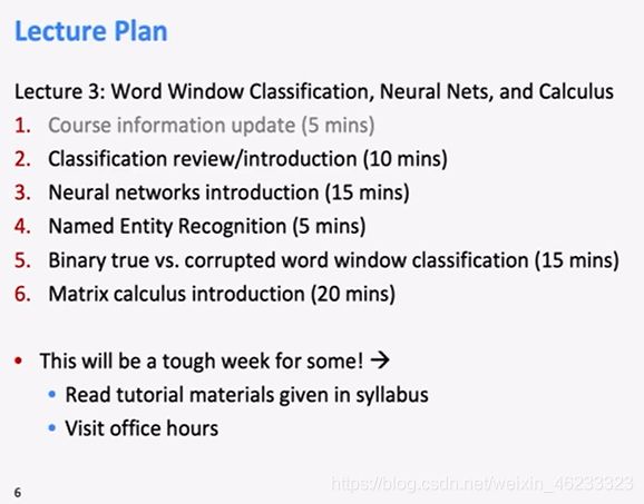
Little new knowledge in this lecture.

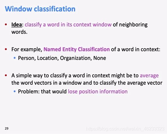
Binary word window classification

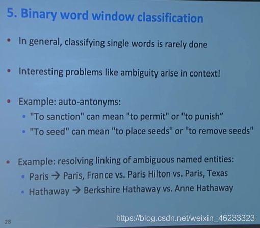
Use the window of word to classifiy the center word:

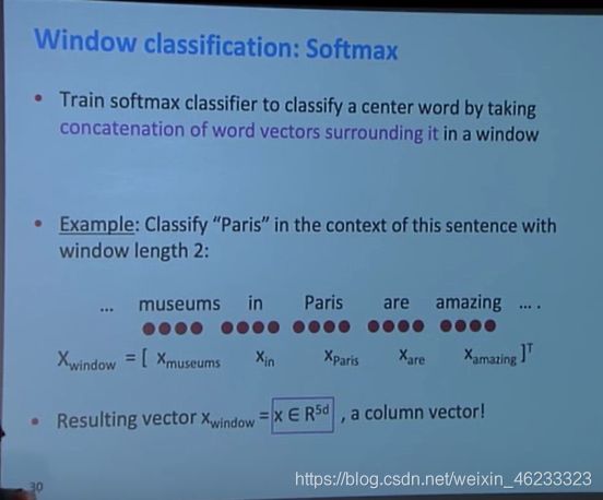
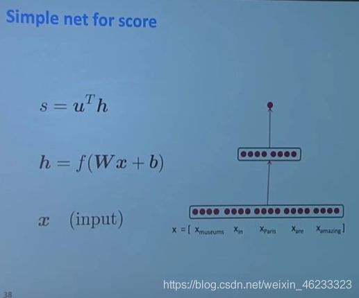
With this bigger vector, we get:

Lecture Four

“In 2019, deeplearrning is still a kind of craft.”

I write the mtrix derivation skills here

附录

常见单词统计

zilch n. 零无价值的物品; 人名
Notation n. 符号;乐谱;计数法
Orthogonality n. 正交性
Determinant n. 决定因素；行列式 adj. 决定性的

相关资源

非常基础的SVD推导
矩阵求导术