Tensorflow笔记——第二讲:神经网络优化
目录
- 2.1 预备知识
- 2.1.1 tf.where()函数:
- 2.1.2 np.random.RandomState.rand()返回一个[0,1)之间的随机数:
- 2.1.3 np.vstack() 将两个数组按垂直方向叠加:
- 2.1.4 np.mgrid[ ] 、.ravel( ) 、np.c_[ ]三个函数结合使用,生成网格坐标点:
- 2.2 神经网络(NN)复杂度学习率
- 2.1.1 神经网络(NN)复杂度:
- 2.2.2 学习率
- 2.3 激活函数
- 2.3.1 Sigmoid激活函数:
- 2.3.2 Tanh激活函数:
- 2.3.3 Relu激活函数:
- 2.3.4 Leaky Relu激活函数,为解决Relu在负区间梯度消失:
- 2.4 损失函数
- 2.4.1 均方误差mse:
- 2.4.2 自定义损失函数:
- 2.4.3 交叉熵损失函数CE(Cross Entropy):表征两个概率分布之间的距离:
- 2.4.4 softmax与交叉熵结合:
- 2.5 缓解过拟合
- 2.5.1 什么是欠拟合与过拟合:
- 2.5.2 欠拟合与过拟合解决方案:
- 2.5.3 正则化缓解过拟合:
- 2.6 优化器
- 2.6.1 神经网络参数优化器:
- 2.6.2 随机梯度下降:SGD(无momentum,也就是不含动量)
- 2.6.3 SGDM(含momentum的SGD),在SGD基础上增加一阶动量
- 2.6.4 Adagrad,在SGD基础上增加二阶动量
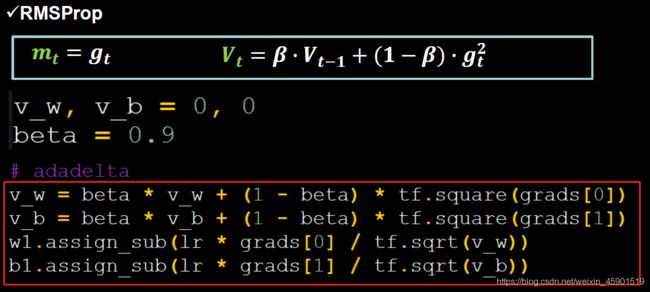
- 2.6.5 RMSProp,SGD基础上增加二阶动量
- 2.6.6 Adam, 同时结合SGDM一阶动量和RMSProp二阶动量
2.1 预备知识
2.1.1 tf.where()函数:

上面的tf.greater(a,b)函数:
功能:比较a、b两个值的大小
返回值:一个列表,元素值都是true和false。如上面应该返回tf.Tensor([ True True False False False], shape=(5,), dtype=bool)
2.1.2 np.random.RandomState.rand()返回一个[0,1)之间的随机数:

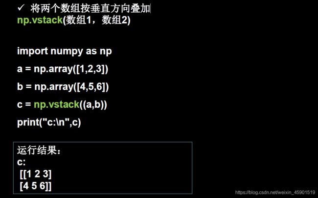
2.1.3 np.vstack() 将两个数组按垂直方向叠加:
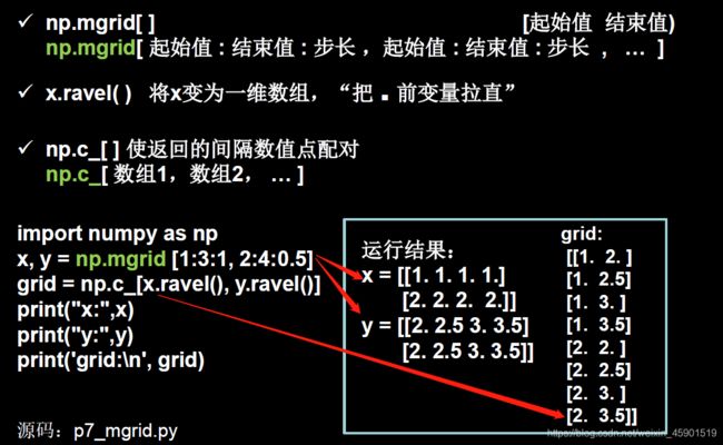
2.1.4 np.mgrid[ ] 、.ravel( ) 、np.c_[ ]三个函数结合使用,生成网格坐标点:
下面的x为了和y维度一致,所以扩充了。
2.2 神经网络(NN)复杂度学习率
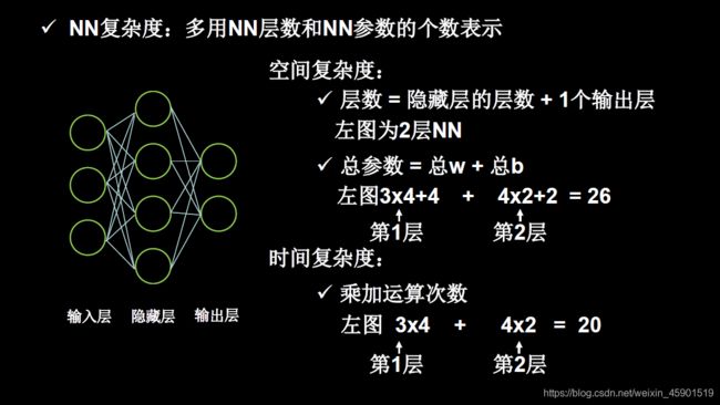
2.1.1 神经网络(NN)复杂度:
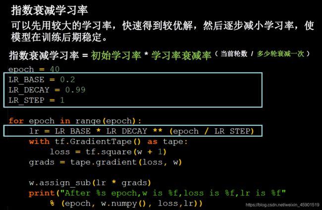
2.2.2 学习率

那设置什么样的学习率比较好呢,或者说学习率怎么设置?
使用指数衰减学习率来解决,下面公式中绿色的是超参数,其中 “学习衰减率 ” 是指学习率按这个比例减小,注意后面括号中的在这个 “学习衰减率 ”的指数上:
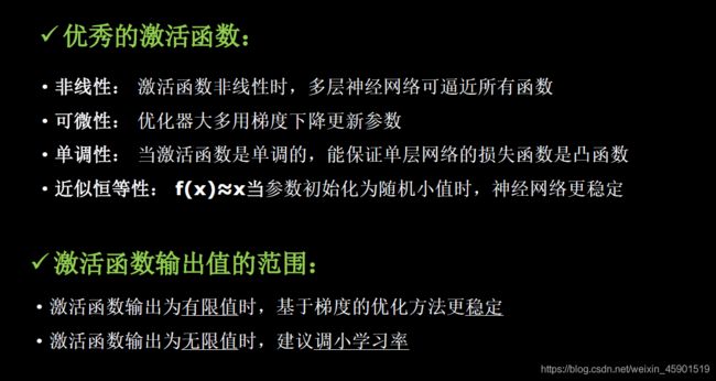
2.3 激活函数
激活函数的加入提升了模型的表达能力。
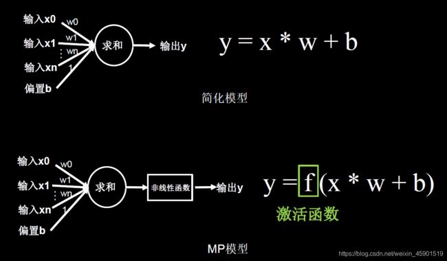
下面看看常用的激活函数:
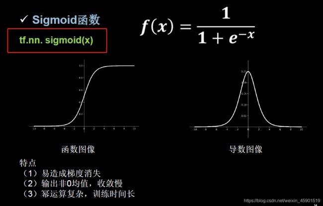
2.3.1 Sigmoid激活函数:
2.3.2 Tanh激活函数:

2.3.3 Relu激活函数:

2.3.4 Leaky Relu激活函数,为解决Relu在负区间梯度消失:


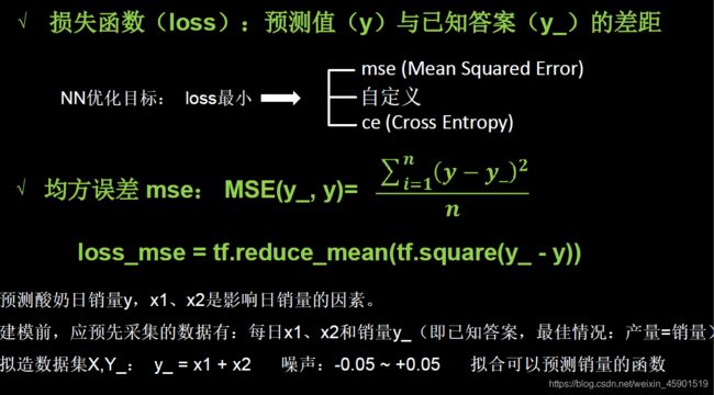
2.4 损失函数
2.4.1 均方误差mse:
上面例子的代码如下:
import tensorflow as tf
import numpy as np

SEED = 23455

rdm = np.random.RandomState(seed=SEED)  # 生成[0,1)之间的随机数
x = rdm.rand(32, 2)
y_ = [[x1 + x2 + (rdm.rand() / 10.0 - 0.05)] for (x1, x2) in x]  # 生成噪声[0,1)/10=[0,0.1); [0,0.1)-0.05=[-0.05,0.05)
x = tf.cast(x, dtype=tf.float32)

w1 = tf.Variable(tf.random.normal([2, 1], stddev=1, seed=1))

epoch = 15000
lr = 0.002

for epoch in range(epoch):
    with tf.GradientTape() as tape:
        y = tf.matmul(x, w1)
        loss_mse = tf.reduce_mean(tf.square(y_ - y))

    grads = tape.gradient(loss_mse, w1)  # 计算w1的梯度
    w1.assign_sub(lr * grads)   # 更新参数w1

    if epoch % 500 == 0:
        print("After %d training steps,w1 is " % (epoch))
        print(w1.numpy(), "\n")
print("Final w1 is: ", w1.numpy())
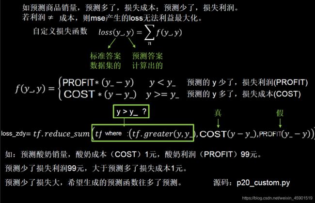
2.4.2 自定义损失函数:
MSE损失默认损失的成本和损失的利润是一样的,但实际上是不一样的,这时就需要自定义损失函数了。
代码如下:
import tensorflow as tf
import numpy as np

SEED = 23455
COST = 1
PROFIT = 99

rdm = np.random.RandomState(SEED)
x = rdm.rand(32, 2)
y_ = [[x1 + x2 + (rdm.rand() / 10.0 - 0.05)] for (x1, x2) in x]  # 生成噪声[0,1)/10=[0,0.1); [0,0.1)-0.05=[-0.05,0.05)
x = tf.cast(x, dtype=tf.float32)

w1 = tf.Variable(tf.random.normal([2, 1], stddev=1, seed=1))

epoch = 10000
lr = 0.002

for epoch in range(epoch):
    with tf.GradientTape() as tape:
        y = tf.matmul(x, w1)
        loss = tf.reduce_sum(tf.where(tf.greater(y, y_), (y - y_) * COST, (y_ - y) * PROFIT))

    grads = tape.gradient(loss, w1)
    w1.assign_sub(lr * grads)

    if epoch % 500 == 0:
        print("After %d training steps,w1 is " % (epoch))
        print(w1.numpy(), "\n")
print("Final w1 is: ", w1.numpy())

# 自定义损失函数
# 酸奶成本1元, 酸奶利润99元
# 成本很低,利润很高,人们希望多预测些,生成模型系数大于1,往多了预测
2.4.3 交叉熵损失函数CE(Cross Entropy):表征两个概率分布之间的距离:

tensorflow是这样写交叉熵损失函数的,看下面:

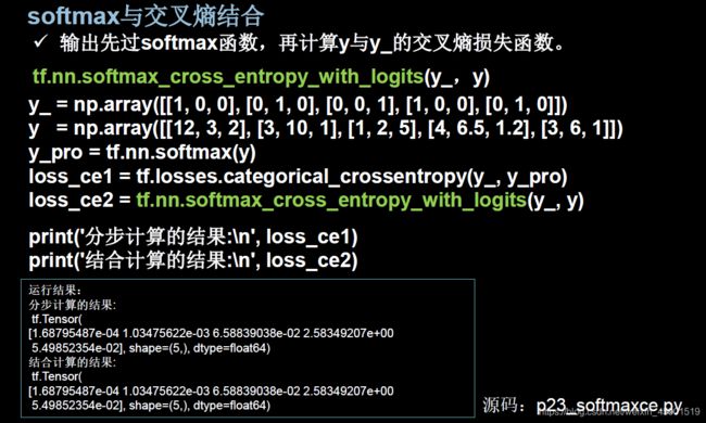
2.4.4 softmax与交叉熵结合:
2.5 缓解过拟合
2.5.1 什么是欠拟合与过拟合:

2.5.2 欠拟合与过拟合解决方案:

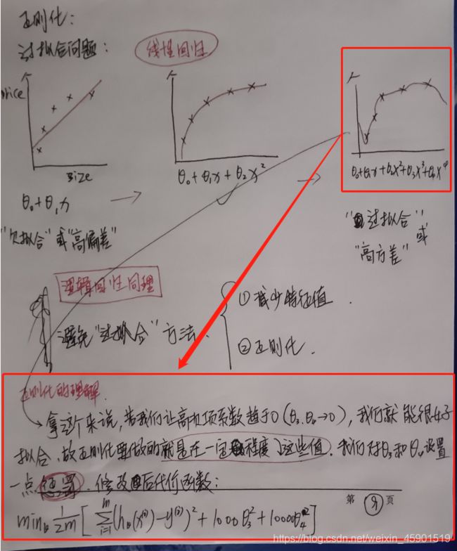
2.5.3 正则化缓解过拟合:
首先要知道什么是正则化,这里我把以前手写的吴恩达老师课程的笔记放在这里,加深理解:


下面看看L2正则化计算Loss w的过程:

用一个实际的例子来说明,下面的数据有两个输入特征和一个输出标签,用已知数据训练一个神经网络,来判断在未知数据上的标签是0还是1。
数据:
链接:https://pan.baidu.com/s/18U-rjPk3zi9IbdF-tuTxEA
提取码:cyc2
思路是这样的:先用神经网络拟合出标签x1、x2与标签y_c的函数关系;然后以x1、x2作为横纵坐标可视化这些点,生成网格覆盖这些点;再把这些网络的交点,也就是横纵坐标作为输入送入训练好的神经网络,神经网络会为每个坐标输出一个预测值。我们要区分输出偏向1还是0,可以把神经网络输出的预测值为0.5的线标出颜色,这条线就是0和1的区分线了。

没使用正则化的代码以及可视化结果:
# 导入所需模块
import tensorflow as tf
from matplotlib import pyplot as plt
import numpy as np
import pandas as pd

# 读入数据/标签 生成x_train y_train
df = pd.read_csv('dot.csv')
x_data = np.array(df[['x1', 'x2']])
y_data = np.array(df['y_c'])

x_train = np.vstack(x_data).reshape(-1, 2)
y_train = np.vstack(y_data).reshape(-1, 1)

Y_c = [['red' if y else 'blue'] for y in y_train]

# 转换x的数据类型,否则后面矩阵相乘时会因数据类型问题报错
x_train = tf.cast(x_train, tf.float32)
y_train = tf.cast(y_train, tf.float32)

# from_tensor_slices函数切分传入的张量的第一个维度,生成相应的数据集,使输入特征和标签值一一对应
train_db = tf.data.Dataset.from_tensor_slices((x_train, y_train)).batch(32)

# 生成神经网络的参数,输入层为2个神经元,隐藏层为11个神经元,1层隐藏层,输出层为1个神经元
# 用tf.Variable()保证参数可训练
w1 = tf.Variable(tf.random.normal([2, 11]), dtype=tf.float32)
b1 = tf.Variable(tf.constant(0.01, shape=[11]))

w2 = tf.Variable(tf.random.normal([11, 1]), dtype=tf.float32)
b2 = tf.Variable(tf.constant(0.01, shape=[1]))

lr = 0.005  # 学习率
epoch = 800  # 循环轮数

# 训练部分
for epoch in range(epoch):
    for step, (x_train, y_train) in enumerate(train_db):
        with tf.GradientTape() as tape:  # 记录梯度信息

            h1 = tf.matmul(x_train, w1) + b1  # 记录神经网络乘加运算
            h1 = tf.nn.relu(h1)
            y = tf.matmul(h1, w2) + b2

            # 采用均方误差损失函数mse = mean(sum(y-out)^2)
            loss = tf.reduce_mean(tf.square(y_train - y))

        # 计算loss对各个参数的梯度
        variables = [w1, b1, w2, b2]
        grads = tape.gradient(loss, variables)

        # 实现梯度更新
        # w1 = w1 - lr * w1_grad tape.gradient是自动求导结果与[w1, b1, w2, b2] 索引为0,1,2,3
        w1.assign_sub(lr * grads[0])
        b1.assign_sub(lr * grads[1])
        w2.assign_sub(lr * grads[2])
        b2.assign_sub(lr * grads[3])

    # 每20个epoch,打印loss信息
    if epoch % 20 == 0:
        print('epoch:', epoch, 'loss:', float(loss))

# 预测部分
print("*******predict*******")
# xx在-3到3之间以步长为0.01,yy在-3到3之间以步长0.01,生成间隔数值点
xx, yy = np.mgrid[-3:3:.1, -3:3:.1]
# 将xx , yy拉直,并合并配对为二维张量,生成二维坐标点
grid = np.c_[xx.ravel(), yy.ravel()]
grid = tf.cast(grid, tf.float32)
# 将网格坐标点喂入神经网络,进行预测,probs为输出
probs = []
for x_test in grid:
    # 使用训练好的参数进行预测
    h1 = tf.matmul([x_test], w1) + b1
    h1 = tf.nn.relu(h1)
    y = tf.matmul(h1, w2) + b2  # y为预测结果
    probs.append(y)

# 取第0列给x1,取第1列给x2
x1 = x_data[:, 0]
x2 = x_data[:, 1]
# probs的shape调整成xx的样子
probs = np.array(probs).reshape(xx.shape)
plt.scatter(x1, x2, color=np.squeeze(Y_c))  # squeeze去掉纬度是1的纬度,相当于去掉[['red'],[''blue]],内层括号变为['red','blue']
# 把坐标xx yy和对应的值probs放入contour函数,给probs值为0.5的所有点上色  plt.show()后 显示的是红蓝点的分界线
plt.contour(xx, yy, probs, levels=[.5])
plt.show()

# 读入红蓝点,画出分割线,不包含正则化
# 不清楚的数据,建议print出来查看
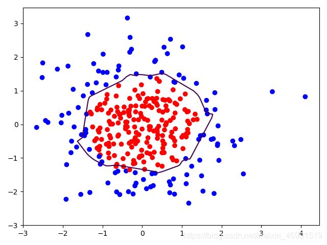
可看到轮廓不够平滑,存在过拟合现象。
正则化预测代码及可视化:
# 导入所需模块
import tensorflow as tf
from matplotlib import pyplot as plt
import numpy as np
import pandas as pd

# 读入数据/标签 生成x_train y_train
df = pd.read_csv('dot.csv')
x_data = np.array(df[['x1', 'x2']])
y_data = np.array(df['y_c'])

x_train = x_data
y_train = y_data.reshape(-1, 1)

Y_c = [['red' if y else 'blue'] for y in y_train]

# 转换x的数据类型,否则后面矩阵相乘时会因数据类型问题报错
x_train = tf.cast(x_train, tf.float32)
y_train = tf.cast(y_train, tf.float32)

# from_tensor_slices函数切分传入的张量的第一个维度,生成相应的数据集,使输入特征和标签值一一对应
train_db = tf.data.Dataset.from_tensor_slices((x_train, y_train)).batch(32)

# 生成神经网络的参数,输入层为4个神经元,隐藏层为32个神经元,2层隐藏层,输出层为3个神经元
# 用tf.Variable()保证参数可训练
w1 = tf.Variable(tf.random.normal([2, 11]), dtype=tf.float32)
b1 = tf.Variable(tf.constant(0.01, shape=[11]))

w2 = tf.Variable(tf.random.normal([11, 1]), dtype=tf.float32)
b2 = tf.Variable(tf.constant(0.01, shape=[1]))

lr = 0.005  # 学习率为
epoch = 800  # 循环轮数

# 训练部分
for epoch in range(epoch):
    for step, (x_train, y_train) in enumerate(train_db):
        with tf.GradientTape() as tape:  # 记录梯度信息

            h1 = tf.matmul(x_train, w1) + b1  # 记录神经网络乘加运算
            h1 = tf.nn.relu(h1)
            y = tf.matmul(h1, w2) + b2

            # 采用均方误差损失函数mse = mean(sum(y-out)^2)
            loss_mse = tf.reduce_mean(tf.square(y_train - y))
            # 添加l2正则化
            loss_regularization = []
            # tf.nn.l2_loss(w)=sum(w ** 2) / 2
            loss_regularization.append(tf.nn.l2_loss(w1))
            loss_regularization.append(tf.nn.l2_loss(w2))
            # 求和
            # 例:x=tf.constant(([1,1,1],[1,1,1]))
            #   tf.reduce_sum(x)
            # >>>6
            loss_regularization = tf.reduce_sum(loss_regularization)
            loss = loss_mse + 0.03 * loss_regularization  # REGULARIZER = 0.03

        # 计算loss对各个参数的梯度
        variables = [w1, b1, w2, b2]
        grads = tape.gradient(loss, variables)

        # 实现梯度更新
        # w1 = w1 - lr * w1_grad
        w1.assign_sub(lr * grads[0])
        b1.assign_sub(lr * grads[1])
        w2.assign_sub(lr * grads[2])
        b2.assign_sub(lr * grads[3])

    # 每200个epoch,打印loss信息
    if epoch % 20 == 0:
        print('epoch:', epoch, 'loss:', float(loss))

# 预测部分
print("*******predict*******")
# xx在-3到3之间以步长为0.01,yy在-3到3之间以步长0.01,生成间隔数值点
xx, yy = np.mgrid[-3:3:.1, -3:3:.1]
# 将xx, yy拉直,并合并配对为二维张量,生成二维坐标点
grid = np.c_[xx.ravel(), yy.ravel()]
grid = tf.cast(grid, tf.float32)
# 将网格坐标点喂入神经网络,进行预测,probs为输出
probs = []
for x_predict in grid:
    # 使用训练好的参数进行预测
    h1 = tf.matmul([x_predict], w1) + b1
    h1 = tf.nn.relu(h1)
    y = tf.matmul(h1, w2) + b2  # y为预测结果
    probs.append(y)

# 取第0列给x1,取第1列给x2
x1 = x_data[:, 0]
x2 = x_data[:, 1]
# probs的shape调整成xx的样子
probs = np.array(probs).reshape(xx.shape)
plt.scatter(x1, x2, color=np.squeeze(Y_c))
# 把坐标xx yy和对应的值probs放入contour函数,给probs值为0.5的所有点上色  plt.show()后 显示的是红蓝点的分界线
plt.contour(xx, yy, probs, levels=[.5])
plt.show()

# 读入红蓝点,画出分割线,包含正则化
# 不清楚的数据,建议print出来查看

从图片可以看出,曲线平滑,有效缓解了过拟合现象。
2.6 优化器
优化器是引导神经网络更新参数的工具。优化算法可以分成一阶优化和二阶优化算法,其中一阶优化就是指的梯度算法及其变种,而二阶优化一般是用二阶导数(Hessian 矩阵)来计算,如牛顿法,由于需要计算Hessian阵和其逆矩阵,计算量较大,因此没有流行开来。这里主要总结一阶优化的各种梯度下降方法。
深度学习优化算法经历了SGD -> SGDM -> NAG ->AdaGrad -> AdaDelta -> Adam -> Nadam这样的发展历程。
2.6.1 神经网络参数优化器:
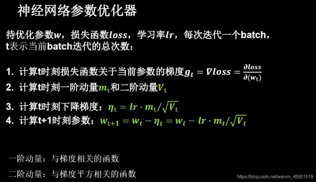
上述的,步骤3,4对于各算法都是一致的,主要差别体现在步骤1和2上。
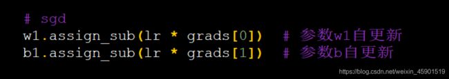
2.6.2 随机梯度下降:SGD(无momentum,也就是不含动量)

tensorflow代码实现:
2.6.3 SGDM(含momentum的SGD),在SGD基础上增加一阶动量

代码实现是下面这面这样:

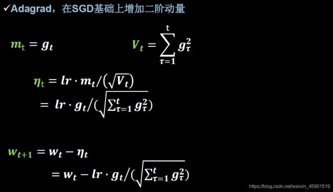
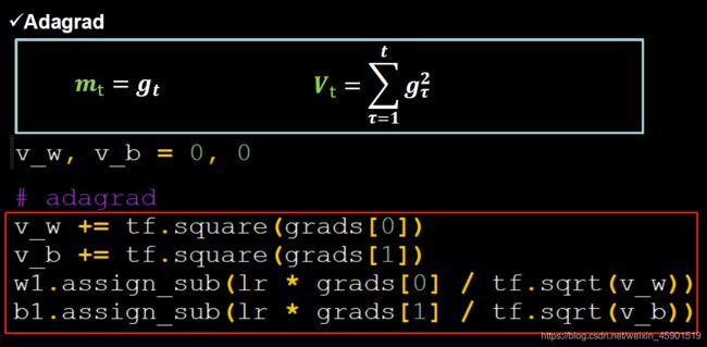
2.6.4 Adagrad,在SGD基础上增加二阶动量
代码实现:
2.6.5 RMSProp,SGD基础上增加二阶动量

代码实现:
2.6.6 Adam, 同时结合SGDM一阶动量和RMSProp二阶动量

代码实现:
