吴恩达机器学习作业——逻辑回归
1 Logistic regression
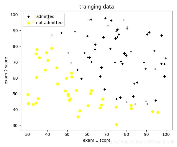
在这部分的练习中,你将建立一个逻辑回归模型来预测一个学生是否能进入大学。假设你是一所大学的行政管理人员,你想根据两门考试的结果,来决定每个申请人是否被录取。你有以前申请人的历史数据,可以将其用作逻辑回归训练集。对于每一个训练样本,你有申请人两次测评的分数以及录取的结果。为了完成这个预测任务,我们准备构建一个可以基于两次测试评分来评估录取可能性的分类模型。
1.1 Visualizing the data
在开始实施算法之前,最好将数据可视化
添加库
import pandas as pd
import matplotlib.pyplot as plt
import numpy as np
from sklearn.metrics import classification_report
读取训练集数据
path = 'ex2data1.txt'
data = pd.read_csv(path, header=None, names=['exam 1 score', 'exam 2 score', 'admitted'])
# print(data.head())
# print(data.describe())
将正向类和负向类以散点图形式画出
# 将录取和未录取数据分开
positive = data[data.admitted.isin(['1'])]
negative = data[data.admitted.isin(['0'])]

# 可视化训练集数据
fig, ax = plt.subplots(figsize=(6, 5))
ax.scatter(positive['exam 1 score'], positive['exam 2 score'], c='black', marker='+', label='admitted')
ax.scatter(negative['exam 1 score'], negative['exam 2 score'], c='yellow', marker='o', label='not admitted')
ax.legend(loc=2)  # 数据点注释
ax.set_xlabel('exam 1 score')
ax.set_ylabel('exam 2 score')
ax.set_title('trainging data')
1.2 sigmoid 函数
def sigmoid(x):
    return np.exp(x) / (1 + np.exp(x))
1.3 代价函数
def computecost(X, y, theta):
    theta = np.matrix(theta)
    X = np.matrix(X)
    y = np.matrix(y)
    first = np.multiply(-y, np.log(sigmoid(np.dot(X, theta.T))))
    second = np.multiply((1 - y), np.log(1 - sigmoid(np.dot(X, theta.T))))
    return np.sum(first - second) / (len(X))
1.4 梯度下降
def gradientdescent(X, y, theta, alpha, epoch):
    temp = np.matrix(np.zeros(theta.shape))
    m = X.shape[0]
    cost = np.zeros(epoch)

    for i in range(epoch):
        A = sigmoid(np.dot(X, theta.T))
        temp = theta - (alpha / m) * (A - y).T * X
        theta = temp
        cost[i] = computecost(X, y, theta)

    return theta, cost
1.5 训练 theta 参数
在训练之前先将学生成绩进行归一化处理
data.insert(0, 'Ones', 100)
cols = data.shape[1]  # 列数
X = data.iloc[:, 0:cols - 1]
y = data.iloc[:, cols - 1:cols]
# theta = np.zeros(X.shape[1])
theta = np.ones(3)
X = np.matrix(X)
X = X / 100  # 归一化
y = np.matrix(y)
theta = np.matrix(theta)
训练开始
alpha = 0.3
epoch = 100000
origin_cost = computecost(X, y, theta)
final_theta, cost = gradientdescent(X, y, theta, alpha, epoch)
输出 theta 参数
print(final_theta)
# [[-24.99361363  20.48877093  20.01095566]]
1.6 评估算法
预测函数,输入学生成绩,输出录取的概率
def predict(theta, X):
    probability = sigmoid(np.dot(X, theta.T))
    return [1 if x >= 0.5 else 0 for x in probability]
检验正确率
predictions = predict(final_theta, X)
correct = [1 if a == b else 0 for (a, b) in zip(predictions, y)]
accuracy = sum(correct) / len(X)
print(accuracy)
# 输出 0.89
或者用 sklearn 中的方法来检验
from sklearn.metrics import classification_report
print(classification_report(predictions, y))
              precision    recall  f1-score   support

           0       0.85      0.87      0.86        39
           1       0.92      0.90      0.91        61

    accuracy                           0.89       100
   macro avg       0.88      0.89      0.88       100
weighted avg       0.89      0.89      0.89       100
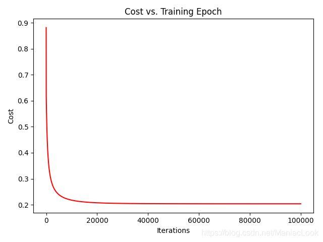
代价函数变化
fig, ax = plt.subplots()
ax.plot(np.arange(epoch), cost, 'r')
ax.set_xlabel('Iterations')
ax.set_ylabel('Cost')
ax.set_title('Cost vs. Training Epoch')
plt.show()
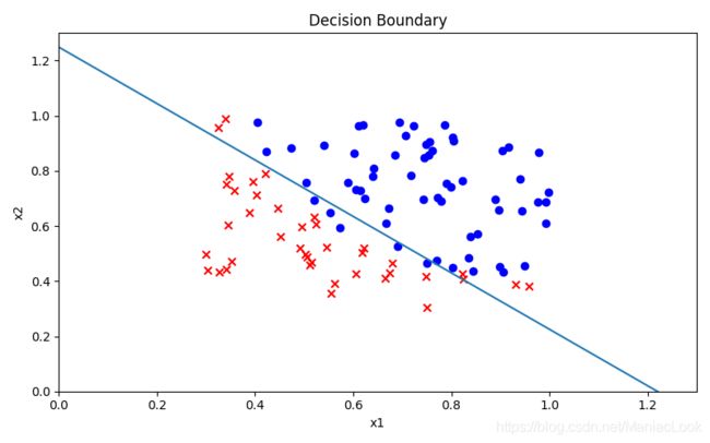
1.7 决策边界
![]()
x1 = np.arange(1.3, step=0.01)
x2 = -(final_theta[0, 0] + x1 * final_theta[0, 1]) / final_theta[0, 2]

fig, ax = plt.subplots(figsize=(8, 5))
ax.scatter(positive['exam 1 score'] / 100, positive['exam 2 score'] / 100, c='b', label='Admitted')
ax.scatter(negative['exam 1 score'] / 100, negative['exam 2 score'] / 100, c='r', marker='x', label='Not Admitted')
ax.plot(x1, x2)
ax.set_xlim(0, 1.3)
ax.set_ylim(0, 1.3)
ax.set_xlabel('x1')
ax.set_ylabel('x2')
ax.set_title('Decision Boundary')
plt.show()
决策边界图
2 Regularized logistic regression
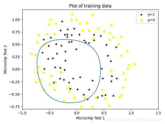
在这部分练习中,您将实现正则化逻辑回归,以预测制造厂的微芯片是否通过质量保证(QA)。在QA过程中,每个微芯片都要经过各种测试,以确保其正常工作。
假设你是工厂的产品经理,你有对一些微芯片的测试结果进行了两次不同的测试。从这两个测试中,您想确定是否应该接受或拒绝微芯片。为了帮助你做出决定,你有一个过去芯片测试结果的数据集,从中你可以建立一个逻辑回归模型。
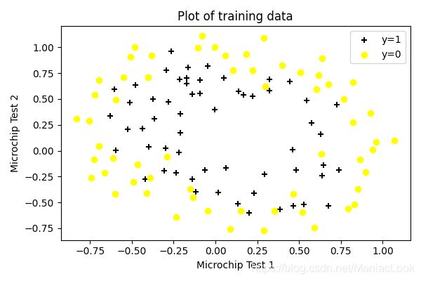
2.1 Visualizing the data
先读取训练集
data = pd.read_csv('ex2data2.txt', names=['Test 1', 'Test 2', 'Accepted'])
print(data.head())
print(data.describe())
输出结果
     Test 1   Test 2  Accepted
0  0.051267  0.69956         1
1 -0.092742  0.68494         1
2 -0.213710  0.69225         1
3 -0.375000  0.50219         1
4 -0.513250  0.46564         1
           Test 1      Test 2    Accepted
count  118.000000  118.000000  118.000000
mean     0.054779    0.183102    0.491525
std      0.496654    0.519743    0.502060
min     -0.830070   -0.769740    0.000000
25%     -0.372120   -0.254385    0.000000
50%     -0.006336    0.213455    0.000000
75%      0.478970    0.646562    1.000000
max      1.070900    1.108900    1.000000
然后画图
# 数据分类
positive = data[data.Accepted.isin(['1'])]
negative = data[data.Accepted.isin(['0'])]

# 可视化数据
fig, ax = plt.subplots(figsize=(6, 4))
ax.scatter(positive['Test 1'], positive['Test 2'], c='black', marker='+', label='y=1')
ax.scatter(negative['Test 1'], negative['Test 2'], c='yellow', marker='o', label='y=0')
ax.legend(loc=1)
ax.set_xlabel('Microchip Test 1')
ax.set_ylabel('Microchip Test 2')
ax.set_title('Plot of training data')
plt.show()
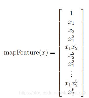
2.2 Feature mapping
更好地拟合数据的一种方法是从每个数据点创建更多的特征。我们将把特征映射为 x1 和 x2 的所有多项式项,直到六次方。即计算 (1 + x1 + x2 + x12 + x1x2 + x22 + … + x1x25 + x26)
# 特征映射
def feature_mapping(x1, x2, power):
    data2 = {}
    for i in np.arange(power + 1):
        for p in np.arange(i + 1):
            data2["f{}{}".format(i - p, p)] = np.power(x1, i - p) * np.power(x2, p)
    return pd.DataFrame(data2)


# 计算6阶的特征映射
x1 = data['Test 1'].values
x2 = data['Test 2'].values
data2 = feature_mapping(x1, x2, 6)
print(data2.head())
   f00       f10      f01       f20  ...       f33       f24       f15       f06
0  1.0  0.051267  0.69956  0.002628  ...  0.000046  0.000629  0.008589  0.117206
1  1.0 -0.092742  0.68494  0.008601  ... -0.000256  0.001893 -0.013981  0.103256
2  1.0 -0.213710  0.69225  0.045672  ... -0.003238  0.010488 -0.033973  0.110047
3  1.0 -0.375000  0.50219  0.140625  ... -0.006679  0.008944 -0.011978  0.016040
4  1.0 -0.513250  0.46564  0.263426  ... -0.013650  0.012384 -0.011235  0.010193
作为这个映射的结果,我们的两个特征向量(两个QA测试的分数)被转换成28维向量。在这个高维特征向量上训练的logistic回归分类器将具有更复杂的决策边界,并且在我们的二维图中绘制时将出现非线性。
虽然特征映射允许我们构建更具表现力的分类器,但它也更容易过度拟合。在练习的下一部分中,您将实现正则化logistic回归来拟合数据,还将亲眼看看正则化如何帮助解决过度拟合问题。
2.3 Cost function and gradient
现在实现代码来计算正则logistic回归的代价函数和梯度。
回想一下,logistic回归中的正则化成本函数是
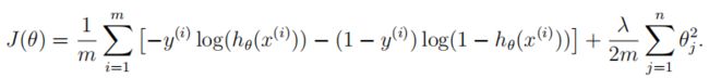
请注意,不应正则化参数θ0。
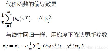
成本函数的梯度是一个向量,其中第j个元素定义如下:
# sigmoid 函数
def sigmoid(x):
    return 1 / (1 + np.exp(-x))


# 代价函数
def cost(theta, X, y):
    first = (-y) * np.log(sigmoid(X @ theta))
    second = (1 - y) * np.log(1 - sigmoid(X @ theta))
    return np.mean(first - second)


# 正则化代价函数
def costreg(theta, X, y, learningrate):
    _theta = theta[1:]
    reg = (learningrate / (2 * len(X))) * (_theta @ _theta)
    return cost(theta, X, y) + reg
# 梯度
def gradient(theta, X, y):
    return (X.T @ (sigmoid(X @ theta) - y)) / len(X)


# 正则化梯度
def gradientreg(theta, X, y, learningrate):
    reg = (learningrate / len(X)) * theta
    reg[0] = 0  # 不惩罚θ0
    return gradient(theta, X, y) + reg
2.4 训练参数 θ
获得训练集和初始化 θ 为 0
X = data2.values
y = data['Accepted'].values
theta = np.zeros(X.shape[1])
print(X.shape, y.shape, theta.shape)
print(costreg(theta, X, y, 1))
(118, 28) (118,) (28,)
0.6931471805599454
(1)用 fmin_tnc 函数训练
result1 = opt.fmin_tnc(func=costreg, x0=theta, fprime=gradientreg, args=(X, y, 2))
print(result1)
(array([ 1.02253248,  0.56283944,  1.13465456, -1.78529748, -0.66539169,
       -1.01863181,  0.13957059, -0.29358911, -0.30102279, -0.08324363,
       -1.27205982, -0.06137378, -0.53996494, -0.17881798, -0.94198718,
       -0.14054843, -0.17736659, -0.07697368, -0.22918936, -0.21349659,
       -0.37205336, -0.86417647,  0.00890082, -0.26795949, -0.0036225 ,
       -0.28315229, -0.07321593, -0.75992548]), 57, 1)
(2)用 minimize 函数训练
result2 = opt.minimize(fun=costreg, x0=theta, args=(X, y, 2), method='TNC', jac=gradientreg)
print(result2)
fun: 0.5830356764058148
     jac: array([0.00318613, 0.00371841, 0.01438163, 0.00439174, 0.0042439 ,
       0.01363881, 0.0025095 , 0.00300901, 0.00121719, 0.01128844,
       0.00351398, 0.00083453, 0.00220748, 0.00131178, 0.0112205 ,
       0.00258022, 0.00113796, 0.00020022, 0.0017479 , 0.00077718,
       0.00942953, 0.00305894, 0.00032368, 0.0007994 , 0.00012105,
       0.00142873, 0.00056985, 0.00951201])
 message: 'Converged (|f_n-f_(n-1)| ~= 0)'
    nfev: 57
     nit: 2
  status: 1
 success: True
       x: array([ 1.02253248,  0.56283944,  1.13465456, -1.78529748, -0.66539169,
       -1.01863181,  0.13957059, -0.29358911, -0.30102279, -0.08324363,
       -1.27205982, -0.06137378, -0.53996494, -0.17881798, -0.94198718,
       -0.14054843, -0.17736659, -0.07697368, -0.22918936, -0.21349659,
       -0.37205336, -0.86417647,  0.00890082, -0.26795949, -0.0036225 ,
       -0.28315229, -0.07321593, -0.75992548])
2.5 Evaluating logistic regression
final_theta = result1[0]
predictions = predict(final_theta, X)
correct = [1 if a == b else 0 for (a, b) in zip(predictions, y)]
accuracy = sum(correct) / len(X)
print(accuracy)

final_theta = result2.x
predictions = predict(final_theta, X)
correct = [1 if a == b else 0 for (a, b) in zip(predictions, y)]
accuracy = sum(correct) / len(X)
print(accuracy)

from sklearn.metrics import classification_report
print(classification_report(y, predictions))
0.8050847457627118
0.8050847457627118

              precision    recall  f1-score   support

           0       0.85      0.75      0.80        60
           1       0.77      0.86      0.81        58

    accuracy                           0.81       118
   macro avg       0.81      0.81      0.80       118
weighted avg       0.81      0.81      0.80       118
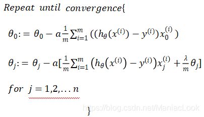
2.6 决策边界
x = np.linspace(-1, 1.5, 250)
xx, yy = np.meshgrid(x, x)

z = feature_mapping(xx.ravel(), yy.ravel(), 6).values
z = z @ final_theta
z = z.reshape(xx.shape)

fig, ax = plt.subplots()
ax.scatter(positive['Test 1'], positive['Test 2'], c='black', marker='+', label='y=1')
ax.scatter(negative['Test 1'], negative['Test 2'], c='yellow', marker='o', label='y=0')
ax.legend(loc=1)
ax.set_xlabel('Microchip Test 1')
ax.set_ylabel('Microchip Test 2')
ax.set_title('Plot of training data')
plt.contour(xx, yy, z, 0)  # 等高线
plt.ylim(-0.8, 1.2)
plt.show()
下图为 λ \lambda λ = 2 时的决策边界
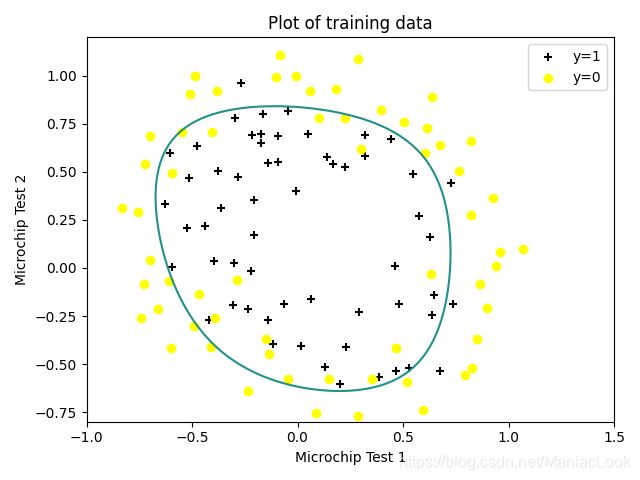
λ \lambda λ = 0 时
λ \lambda λ = 100 时