10_Introduction to Artificial Neural_4_Regression MLP_Sequential_Subclassing_saveMode_Callback_board

10_Introduction to Artificial Neural Networks with Keras_HuberLoss_astype_dtype_DNN_MLP_G.gv.pdf_mnist

https://blog.csdn.net/Linli522362242/article/details/106433059

10_Introduction to Artificial Neural Networks with Keras_2_tensorflow2.1_Anaconda3-2019.10(python3.7.4)
https://blog.csdn.net/Linli522362242/article/details/106537459

10_Introduction to Artificial Neural Networks w Keras_3_FashionMNIST_pydot_sparse_shift(0.)_plt_imgs
https://blog.csdn.net/Linli522362242/article/details/106562190

https://www.cnblogs.com/LittleHann/p/9608599.html#_lab2_1_0 

Building a Regression MLP(Multilayer Perceptron) Using the Sequential API

     Let’s switch to the California housing problem and tackle it using a regression neural network. For simplicity, we will use Scikit-Learn’s fetch_california_housing() function to load the data. This dataset is simpler than the one we used in Cp2
https://blog.csdn.net/Linli522362242/article/details/103387527, since it contains only numerical features (there is no ocean_proximity feature), and there is no missing value. After loading the data, we split it into a training set, a validation set, and a test set, and we scale all the features:

from sklearn.datasets import fetch_california_housing
from sklearn.model_selection import train_test_split
from sklearn.preprocessing import StandardScaler

housing = fetch_california_housing()

 

housing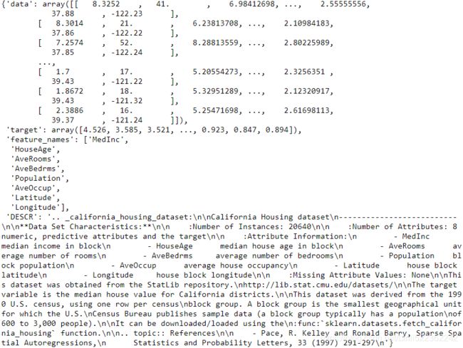

 

pd.DataFrame(housing.data, columns=housing.feature_names).info()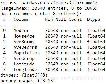

 
Let's load, split and scale the California housing dataset

X_train_full, X_test, y_train_full, y_test = train_test_split( housing.data, housing.target, 
                                                              random_state=42)
X_train, X_valid, y_train, y_valid = train_test_split( X_train_full, y_train_full, 
                                                      random_state=42)

X_train.shape, X_valid.shape, X_test.shape, y_train.shape, y_valid.shape, y_test.shape

 (         (11610, 8),          (3870, 8),         (5160, 8),           (11610,),              (3870,),            (5160,)   )

pd.DataFrame(X_train_full, columns=housing.feature_names).head()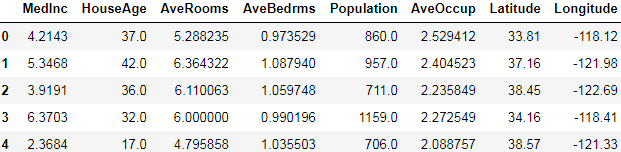

 

https://blog.csdn.net/Linli522362242/article/details/103387527 

     Standardization : first it subtracts the mean value (so standardized values always have a zero mean), and then it divides by the variance so that the resulting distribution has unit variance. 

Machine Learning algorithms don’t perform well when the input numerical attributes have very different scales.

the input numerical attributes have very different scales,  standardization is much less affected by outliers,

scaler = StandardScaler()
X_train = scaler.fit_transform(X_train)
X_valid = scaler.transform(X_valid)
X_test = scaler.transform(X_test)

np.random.seed(42)
tf.random.set_seed(42)

   

https://zhuanlan.zhihu.com/p/38529433/  https://www.sohu.com/a/339641348_701814

http://rishy.github.io/ml/2015/07/28/l1-vs-l2-loss/

使用MAE损失（特别是对于神经网络）的一个大问题是它的梯度始终是相同的，这意味着即使对于小的损失值，其梯度也是大的。这对模型的学习可不好。为了解决这个问题，我们可以使用随着接近最小值而减小的动态学习率。MSE在这种情况下的表现很好，即使采用固定的学习率也会收敛。MSE损失的梯度在Loss较高时会比较大，随着Loss接近0时而下降，从而使其在训练结束时更加精确（参见下图）。

     Using the Sequential API to build, train, evaluate, and use a regression MLP to make predictions is quite similar to what we did for classification. The main differences are the fact that the output layer has a single neuron (since we only want to predict a single value) and uses no activation function, and the loss function is the mean squared error.

https://blog.csdn.net/Linli522362242/article/details/106755312

Using the Sequential API

     Since the dataset is quite noisy, we just use a single hidden layer with fewer neurons than before, to avoid overfitting:

n_hidden = 30 #use a single hidden layer with fewer neurons than before, to avoid overfitting
n_outputs = 1 #the output layer has a single neuron(since we only want to predict a single value)

model = keras.models.Sequential([    #relu max(0,X*w+b)
    keras.layers.Dense( n_hidden, activation="relu", input_shape=X_train.shape[1:] ),
    keras.layers.Dense(n_outputs) # no activation function
])

# After a model is created, you must call its compile() method to specify the loss function 
# and the optimizer to use. 
model.compile( loss="mean_squared_error", optimizer=keras.optimizers.SGD(lr=1e-3) )
keras.utils.plot_model(model, to_file="california_housing_regression_model.png", show_shapes=True)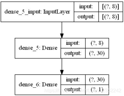

 

history = model.fit( X_train, y_train, epochs=20, validation_data=(X_valid, y_valid))

 

mse_test = model.evaluate( X_test, y_test)
X_new = X_test[:3] # pretend these are new instances
y_pred = model.predict(X_new)

mse_test = model.evaluate( X_test, y_test) 

a lower loss signals a better model

pd.DataFrame( history.history, columns=history.history.keys() ).plot()
plt.grid(True)
#plt.gca().set_ylim(0,1) #
plt.show()

 

pd.DataFrame( history.history, columns=history.history.keys() ).plot()
plt.grid(True)
plt.gca().set_ylim(0,1) #
plt.show()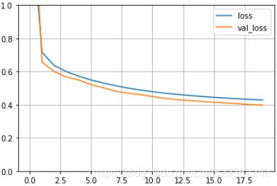

 a lower validation loss signals a better modelhttps://blog.csdn.net/Linli522362242/article/details/106755312

y_pred

 
#https://scikit-learn.org/stable/modules/generated/sklearn.datasets.fetch_california_housing.html
y OR target:    numpy array of shape (20640,):  Each value corresponds to the average house value in units of $100,000

     As you can see, the Sequential API is quite easy to use. However, although Sequential models are extremely common, it is sometimes useful to build neural networks with more complex topologies, or with multiple inputs or outputs. For this purpose, Keras offers the Functional API.

Building Complex Models Using the Functional API

     One example of a nonsequential neural network is a Wide & Deep neural network. This neural network architecture was introduced in a 2016 paper by Heng-Tze Chenget al(https://research.google/pubs/pub45413/). It connects all or part of the inputs directly to the output layer, as shown in Figure 10-14. This architecture makes it possible for the neural network to learn both deep patterns (using the deep path) and simple rules (through the short path). In contrast, a regular MLP forces all the data to flow through the full stack of layers; thus, simple patterns in the data may end up being distorted by this sequence of transformations.

Wide & Deep neural network
  Figure 10-14. Wide & Deep neural network
     Let’s build such a neural network to tackle the California housing problem:

np.random.seed(42)
tf.random.set_seed(42)

# The name input_ is used to avoid overshadowing Python’s built-in input() function
# This is a specification of the kind of input the model will get, including its shape and dtype.
input_ = keras.layers.Input( shape=X_train.shape[1:] )

# Note that we are just telling Keras how it should connect the layers together;
# no actual data is being processed yet.
hidden1 = keras.layers.Dense( 30, activation="relu" )(input_)  #like a function, passing it the input
hidden2 = keras.layers.Dense( 30, activation="relu" )(hidden1) #pass it the output of the first hidden layer

concat = keras.layers.concatenate([input_, hidden2]) #to concatenate the input and the output of the second hidden layer
output = keras.layers.Dense(1)(concat) #passing it the result of the concatenation
model = keras.models.Model( inputs=[input_], outputs=[output])

model.summary()

 concatenate (Concatenate) (None, 38): 38= 30+8

Let’s go through each line of this code:

• First, we need to create an Input object.###The name input_ is used to avoid overshadowing Python’s built-in input() function.### This is a specification of the kind of input the model will get, including its shape and dtype. A model may actually have multiple inputs, as we will see shortly.
   
• Next, we create a Dense layer with 30 neurons, using the ReLU activation function. As soon as it is created, notice that we call it like a function, passing it the input. This is why this is called the Functional API. Note that we are just telling Keras how it should connect the layers together; no actual data is being processed yet.
   
• We then create a second hidden layer, and again we use it as a function. Note that we pass it the output of the first hidden layer.
   
• Next, we create a Concatenate layer, and once again we immediately use it like a function, to concatenate the input and the output of the second hidden layer. You may prefer the keras.layers.concatenate() function, which creates a Concatenate layer and immediately calls it with the given inputs.
   
• Then we create the output layer, with a single neuron and no activation function, and we call it like a function, passing it the result of the concatenation.
   
• Lastly, we create a Keras Model, specifying which inputs and outputs to use.

     Once you have built the Keras model, everything is exactly like earlier, so there’s no need to repeat it here: you must compile the model, train it, evaluate it, and use it to make predictions.

model.compile( loss="mean_squared_error", optimizer=keras.optimizers.SGD(lr=1e-3) )
history = model.fit( X_train, y_train, epochs=20, validation_data=(X_valid, y_valid) )

mse_test = model.evaluate(X_test, y_test)
y_pred = model.predict(X_new)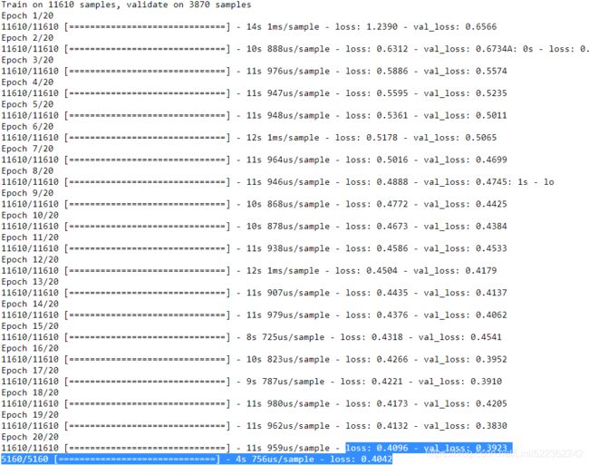

y_pred

send a subset of the features through the wide path and a different subset (possibly overlapping) through the deep path

     But what if you want to send a subset of the features through the wide path and a different subset (possibly overlapping) through the deep path (see Figure 10-15)? In this case, one solution is to use multiple inputs.

  Figure 10-15. Handling multiple inputs

     For example,We will send 5 features (features 0 to 4), and 6 through the deep path (features 2 to 7). Note that 3 features(2,3,4) will go through both (features 2, 3 and 4):

np.random.seed(42)
tf.random.set_seed(42)


input_A = keras.layers.Input( shape=[5], name="wide_input" )
input_B = keras.layers.Input( shape=[6], name="deep_input" )

hidden1 = keras.layers.Dense( 30, activation="relu" )(input_B)
hidden2 = keras.layers.Dense( 30, activation="relu" )(hidden1)
concat = keras.layers.concatenate( [input_A, hidden2] )
output = keras.layers.Dense(1, name="output")(concat)

model = keras.models.Model( inputs=[input_A, input_B], outputs=[output] )#########

model.summary()

     The code is self-explanatory. You should name at least the most important layers, especially when the model gets a bit complex like this. Note that we specified inputs=[input_A, input_B] when creating the model.

     Now we can compile the model as usual, but when we call the fit() method, instead of passing a single input matrix X_train, we must pass a pair of matrices (X_train_A, X_train_B): one per input. ###Alternatively, you can pass a dictionary mapping the input names to the input values, like {"wide_input": X_train_A, "deep_input": X_train_B}. This is especially useful when there are many inputs, to avoid getting the order wrong.### The same is true for X_valid, and also for X_test and X_new when you call evaluate() or predict():

model.compile( loss="mse", optimizer=keras.optimizers.SGD(lr=1e-3) )

X_train_A, X_train_B = X_train[:, :5], X_train[:, 2:]
X_valid_A, X_valid_B = X_valid[:, :5], X_valid[:, 2:]
X_test_A, X_test_B = X_test[:, :5], X_test[:, 2:]
X_new_A, X_new_B = X_test_A[:3], X_test_B[:3]

history = model.fit( ( X_train_A, X_train_B ), y_train, epochs=20, 
                     validation_data=( ( X_valid_A, X_valid_B ), y_valid )
                   )

mse_test = model.evaluate( (X_test_A, X_test_B), y_test )
y_pred = model.predict( (X_new_A, X_new_B) )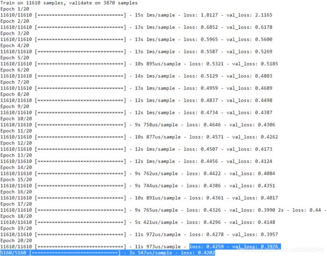

y_pred

multiple outputs

There are many use cases in which you may want to have multiple outputs:

• The task may demand it. For instance, you may want to locate and classify the main object in a picture. This is both a regression task (finding the coordinates of the object’s center, as well as its width and height) and a classification task.
   
• Similarly, you may have multiple independent tasks based on the same data. Sure, you could train one neural network per task, but in many cases you will get better results on all tasks by training a single neural network with one output per task. This is because the neural network can learn features in the data that are useful across tasks. For example, you could perform multitask classification on pictures of faces, using one output to classify the person’s facial expression (smiling, surprised, etc.) and another output to identify whether they are wearing glasses or not.
   
• Another use case is as a regularization technique (i.e., a training constraint whose objective is to reduce overfitting and thus improve the model’s ability to generalize). For example, you may want to add some auxiliary[ɔːɡˈzɪliəri]辅助的 outputs in a neural network architecture (see Figure 10-16) to ensure that the underlying part of the network learns something useful on its own, without relying on the rest of the network.
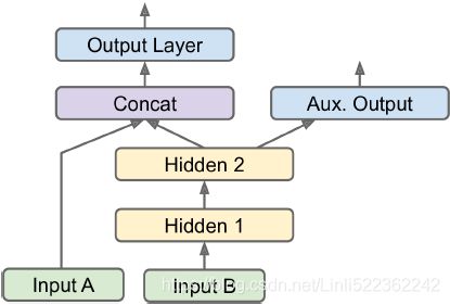  Figure 10-16. Handling multiple outputs, in this example to add an auxiliary output for
  regularization

Adding extra outputs is quite easy: just connect them to the appropriate layers and add them to your model’s list of outputs. For example, the following code builds the network represented in Figure 10-16:

input_A = keras.layers.Input( shape=[5], name="wide_input" ) # 5 features

input_B = keras.layers.Input( shape=[6], name="deep_input" ) # 6 features
hidden1 = keras.layers.Dense( 30, activation="relu", name="hidden1" )(input_B)
hidden2 = keras.layers.Dense( 30, activation="relu", name="hidden2" )(hidden1)

concat = keras.layers.concatenate( [input_A, hidden2] )
output = keras.layers.Dense(1, name="main_output") (concat)

# Adding an auxiliary output for regularization
aux_output = keras.layers.Dense( 1, name="aux_output" )(hidden2)
model = keras.models.Model( inputs=[input_A, input_B], outputs=[output, aux_output] )
model.summary()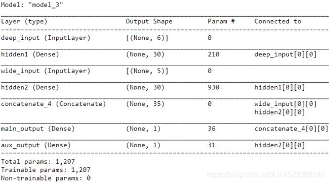

     Each output will need its own loss function. Therefore, when we compile the model, we should pass a list of losses ### Alternatively, you can pass a dictionary that maps each output name to the corresponding loss. Just like for the inputs, this is useful when there are multiple outputs, to avoid getting the order wrong. The loss weights and metrics (discussed shortly) can also be set using dictionaries. ### (if we pass a single loss, Keras will assume that the same loss must be used for all outputs). By default, Keras will compute all these losses and simply add them up to get the final loss used for training. We care much more about the main output than about the auxiliary output (as it is just used for regularization), so we want to give the main output’s loss a much greater weight. Fortunately, it is possible to set all the loss weights when compiling the model:

model.compile( loss=["mse", "mse"], loss_weights=[0.9, 0.1], optimizer=keras.optimizers.SGD(lr=1e-3) )

     Now when we train the model, we need to provide labels for each output. In this example, the main output and the auxiliary output should try to predict the same thing, so they should use the same labels. So instead of passing y_train, we need to pass (y_train, y_train) (and the same goes for y_valid and y_test):

history = model.fit([X_train_A, X_train_B], [y_train, y_train], epochs=20,
                    validation_data=( [X_valid_A, X_valid_B], [y_valid, y_valid] )
                   )

 
... ...

 

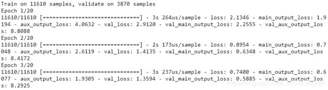
loss(Total)=0.4753 =main_out_loss* loss_weight[0] + aux_output_loss * loss_weight[1] = 0.4245 * 0.9 + 0.9320*0.1

     When we evaluate the model, Keras will return the total loss, as well as all the individual losses:

total_loss, main_loss, aux_loss = model.evaluate( [X_test_A, X_test_B], [y_test, y_test] )
total_loss, main_loss, aux_loss

0.456 = 0.416*0.9 + 0.911 * 0.1

     Similarly, the predict() method will return predictions for each output:

y_pred_main, y_pred_aux = model.predict([X_new_A, X_new_B])
print("y_pred_main: ", y_pred_main,
      "\ny_pred_aux: ", y_pred_aux)

     As you can see, you can build any sort of architecture you want quite easily with the Functional API. Let’s look at one last way you can build Keras models.

Using the Subclassing API to Build Dynamic Models

     Both the Sequential API and the Functional API are declarative: you start by declaring which layers you want to use and how they should be connected, and only then can you start feeding the model some data for training or inference. This has many advantages: the model can easily be saved, cloned, and shared; its structure can be displayed and analyzed; the framework can infer shapes and check types, so errors can be caught early (i.e., before any data ever goes through the model). It’s also fairly easy to debug, since the whole model is a static graph of layers.

      But the flip side is just that: it’s static. Some models involve loops, varying shapes, conditional branching, and other dynamic behaviors. For such cases, or simply if you prefer a more imperative命令的 programming style, the Subclassing API is for you.

     Simply subclass the Model class, create the layers you need in the constructor, and use them to perform the computations you want in the call() method. For example, creating an instance of the following WideAndDeepModel class gives us an equivalent model to the one we just built with the Functional API. You can then compile it, evaluate it, and use it to make predictions, exactly like we just did:

import tensorflow as tf
from tensorflow import keras
from sklearn.datasets import fetch_california_housing
from sklearn.model_selection import train_test_split
from sklearn.preprocessing import StandardScaler

housing = fetch_california_housing()

X_train_full, X_test, y_train_full, y_test = train_test_split( housing.data, housing.target, 
                                                              random_state=42)
X_train, X_valid, y_train, y_valid = train_test_split( X_train_full, y_train_full, 
                                                      random_state=42)

scaler = StandardScaler()
X_train = scaler.fit_transform(X_train)
X_valid = scaler.transform(X_valid)
X_test = scaler.transform(X_test)

X_train_A, X_train_B = X_train[:, :5], X_train[:, 2:]
X_valid_A, X_valid_B = X_valid[:, :5], X_valid[:, 2:]
X_test_A, X_test_B = X_test[:, :5], X_test[:, 2:]

X_new_A, X_new_B = X_test_A[:3], X_test_B[:3]

class WideAndDeepModel( keras.models.Model ):
    def __init__( self, units=30, activation="relu", **kwargs):
        super().__init__(**kwargs) ## handles standard args (e.g., name)
        self.hidden1 = keras.layers.Dense( units, activation=activation )
        self.hidden2 = keras.layers.Dense( units, activation=activation )
        self.main_output = keras.layers.Dense(1)
        self.aux_output = keras.layers.Dense(1)
        
    def call( self, inputs ):
        input_A, input_B = inputs
        
        hidden1 = self.hidden1(input_B)
        hidden2 = self.hidden2(hidden1)
        concat = keras.layers.concatenate([input_A, hidden2])###############
        main_output = self.main_output(concat)
        
        aux_output = self.aux_output(hidden2)
        return main_output, aux_output
        
model = WideAndDeepModel(30, activation="relu")

     This example looks very much like the Functional API,

input_A = keras.layers.Input( shape=[5], name="wide_input" ) # 5 features

input_B = keras.layers.Input( shape=[6], name="deep_input" ) # 6 features
hidden1 = keras.layers.Dense( 30, activation="relu", name="hidden1" )(input_B)
hidden2 = keras.layers.Dense( 30, activation="relu", name="hidden2" )(hidden1)

concat = keras.layers.concatenate( [input_A, hidden2] )
output = keras.layers.Dense(1, name="main_output") (concat)

# Adding an auxiliary output for regularization
aux_output = keras.layers.Dense( 1, name="aux_output" )(hidden2)
model = keras.models.Model( inputs=[input_A, input_B], outputs=[output, aux_output] )
model.summary()

except we do not need to create the inputs###( keras.layers.Input( shape=[5], name="wide_input")  and input_B = keras.layers.Input( shape=[6], name="deep_input" ) )###; we just use the input argument to the call() method, and we separate the creation of the layers####Keras models have an output attribute, so we cannot use that name for the main output layer, which is why we renamed it to main_output.#### in the constructor from their usage in the call() method. The big difference is that you can do pretty much anything you want in the call() method: for loops, if statements, low-level TensorFlow operations—your imagination is the limit (see Chapter 12)! This makes it a great API for researchers experimenting with new ideas.

     This extra flexibility does come at a cost: your model’s architecture is hidden within the call() method, so Keras cannot easily inspect it; it cannot save or clone it; and when you call the summary() method, you only get a list of layers, without any information on how they are connected to each other. Moreover, Keras cannot check types and shapes ahead of time, and it is easier to make mistakes. So unless you really need that extra flexibility, you should probably stick to the Sequential API or the Functional API.

############################

     Keras models can be used just like regular layers, so you can easily combine them to build complex architectures.
############################

# model = WideAndDeepModel(30, activation="relu")
model.compile( loss="mse", loss_weights=[0.9, 0.1], optimizer=keras.optimizers.SGD(lr=1e-3) )
history = model.fit( (X_train_A, X_train_B), (y_train, y_train), epochs=10,
                     validation_data=( (X_valid_A, X_valid_B), (y_valid, y_valid) )
                   )
total_loss, main_loss, aux_loss = model.evaluate( (X_test_A, X_test_B), (y_test, y_test) )
y_pred_main, y_pred_aux = model.predict( (X_new_A, X_new_B) )

 

total_loss, main_loss, aux_loss

(0.5222897731980612, 0.45520294, 1.1322274)  #0.52229 = 0.45520294*0.9 + 1.1322274*0.1

y_pred_main, y_pred_aux

 (array([[0.3183756], [1.6945243], [3.0153322]], dtype=float32),

  array([[1.0351326], [1.6754881], [2.2743428]], dtype=float32)
)

Now that you know how to build and train neural nets using Keras, you will want to save them!

Saving and Restoring a Model

import numpy as np

np.random.seed(42)
tf.random.set_seed(42)

model = keras.models.Sequential([
    keras.layers.Dense(30, activation="relu", input_shape=[8]),
    keras.layers.Dense(30, activation="relu"),
    keras.layers.Dense(1)
]) # # or keras.Model([...])

model.compile( loss="mse", optimizer=keras.optimizers.SGD(lr=1e-3) )
history = model.fit( X_train, y_train, epochs=10, validation_data=(X_valid, y_valid) )
mse_test = model.evaluate(X_test, y_test)

model.save("my_keras_model.h5")

     Keras will use the HDF5 format to

• save both the model’s architecture (including every layer’s hyperparameters) and the values of all the model parameters for every layer (e.g., connection weights and biases).
   
• It also saves the optimizer (including its hyperparameters and any state it may have). In Chapter 19, we will see how to save a tf.keras model using TensorFlow’s SavedModel format instead.

     You will typically have a script that trains a model and saves it, and one or more scripts (or web services) that load the model and use it to make predictions. Loading the model is just as easy:

model = keras.models.load_model("my_keras_model.h5")
X_new= X_test[:3]
model.predict(X_new)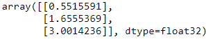

###################################
Note
     This will work when using the Sequential API or the Functional API, but unfortunately not when using model subclassing. You can use save_weights() and load_weights() to at least save and restore the model parameters, but you will need to save and restore everything else yourself.
###################################

model.save_weights("my_keras_weights.ckpt")
model.load_weights("my_keras_weights.ckpt")

     But what if training lasts several hours? This is quite common, especially when training on large datasets. In this case, you should not only save your model at the end of training, but also save checkpoints at regular intervals during training, to avoid losing everything if your computer crashes. But how can you tell the fit() method to save checkpoints? Use callbacks.

Using Callbacks

     The fit() method accepts a callbacks argument that lets you specify a list of objects that Keras will call at the start and end of training, at the start and end of each epoch, and even before and after processing each batch. For example, the ModelCheckpoint callback回调 saves checkpoints of your model at regular intervals during training, by default at the end of each epoch:

keras.backend.clear_session()
np.random.seed(42)
tf.random.set_seed(42)

model = keras.models.Sequential([
    keras.layers.Dense( 30, activation="relu", input_shape=[8] ),
    keras.layers.Dense( 30, activation="relu"),
    keras.layers.Dense(1)
])

# https://www.tensorflow.org/api_docs/python/tf/keras/callbacks/ModelCheckpoint
# mode = "auto"
# 在save_best_only=True时决定性能最佳模型的评判准则，例如，当监测值为val_acc时，模式应为max，
# 当检测值为val_loss时，模式应为min。在auto模式下 mode='auto'，评价准则由被监测值的名字自动推断

#Target: California housing price

model.compile( loss="mse", optimizer=keras.optimizers.SGD(lr = 1e-3) )
# https://www.tensorflow.org/api_docs/python/tf/keras/callbacks/ModelCheckpoint
# mode = "auto"
# monitor='val_loss' #default
checkpoint_cb = keras.callbacks.ModelCheckpoint("my_keras_model.h5", save_best_only=True)###
history = model.fit(X_train, y_train, epochs =10, validation_data=(X_valid, y_valid),
                    callbacks= [checkpoint_cb]
                   )
model = keras.models.load_model("my_keras_model.h5") # rollback to best model
mse_test = model.evaluate( X_test, y_test )

mse_test

     Moreover, if you use a validation set during training, you can set save_best_only=True when creating the ModelCheckpoint. In this case, it will only save your model when its performance on the validation set is the best so far. This way, you do not need to worry about training for too long and overfitting the training set: simply restore the last model saved after training, and this will be the best model on the validation set. The following code is a simple way to implement early stopping (introduced in Cp4 https://blog.csdn.net/Linli522362242/article/details/104124771): 

EarlyStopping + ModelCheckpoint

     Another way to implement early stopping is to simply use the EarlyStopping callback. It will interrupt training when it measures no progress on the validation set for a number of epochs (defined by the patience argument ###Number of epochs with no improvement after which training will be stopped.### ), and it will optionally roll back to the best model. You can combine both callbacks to save checkpoints of your model (in case your computer crashes) and interrupt training early when there is no more progress (to avoid wasting time and resources):

model.compile( loss="mse", optimizer=keras.optimizers.SGD(lr=1e-3) )

# patience: 
#          Number of epochs with no improvement after which training will be stopped.
# restore_best_weights : 
# Whether to restore model weights from the epoch with the best value of the monitored quantity. 
# If False, the model weights obtained at the last step of training are used.

early_stop_cb = keras.callbacks.EarlyStopping(patience = 10, restore_best_weights=True)
checkpoint_cb = keras.callbacks.ModelCheckpoint("my_keras_model.h5", save_best_only=True)

history = model.fit( X_train, y_train, epochs=100, validation_data=(X_valid, y_valid),
                    callbacks=[checkpoint_cb, early_stop_cb]#######
                   )

... ...

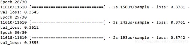
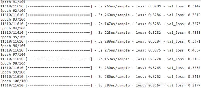
mse_best = model.evaluate(X_test, y_test)

     The number of epochs can be set to a large value since training will stop automatically when there is no more progress. In this case, there is no need to restore the best model saved because the EarlyStopping callback will keep track of the best weights and restore them for you at the end of training.
#############################
     There are many other callbacks available in the keras.callbacks package.
#############################
     If you need extra control, you can easily write your own custom callbacks. As an example of how to do that, the following custom callback will display the ratio between the validation loss and the training loss during training (e.g., to detect overfitting):

class PrintValTrainRatioCallback( keras.callbacks.Callback ):
    def on_epoch_end(self, epoch, logs):
        print("\nval/train: {:.2f}".format( logs["val_loss"]/logs["loss"] ) )

val_train_ratio_cb = PrintValTrainRatioCallback()###########
history = model.fit(X_train, y_train, epochs=1, validation_data=(X_valid, y_valid),
                    callbacks = [val_train_ratio_cb]############
                   )

    As you might expect, you can implement on_train_begin(), on_train_end(), on_epoch_begin(), on_epoch_end(), on_batch_begin(), and on_batch_end(). Callbacks can also be used during evaluation and predictions, should you ever need them (e.g., for debugging).
For evaluation, you should implement on_test_begin(), on_test_end(), on_test_batch_begin(), or on_test_batch_end() (called by evaluate()), and
for prediction you should implement on_predict_begin(), on_predict_end(), on_predict_batch_begin(), or on_predict_batch_end() (called bypredict()).
Now let’s take a look at one more tool you should definitely have in your toolbox when using tf.keras: TensorBoard.

Using TensorBoard for Visualization

     TensorBoard is a great interactive visualization tool that you can use to view the learning curves during training, compare learning curves between multiple runs, visualize the computation graph, analyze training statistics, view images generated by your model, visualize complex multidimensional data projected down to 3D and automatically clustered for you, and more! This tool is installed automatically when you install TensorFlow, so you already have it.

     To use it, you must modify your program so that it outputs the data you want to visualize to special binary log files called event files. Each binary data record is called a summary. The TensorBoard server will monitor the log directory, and it will automatically pick up the changes and update the visualizations: this allows you to visualize live data (with a short delay), such as the learning curves during training. In general, you want to point the TensorBoard server to a root log directory and configure your program so that it writes to a different subdirectory every time it runs. This way, the same TensorBoard server instance will allow you to visualize and compare data from multiple runs of your program, without getting everything mixed up.

     Let’s start by defining the root log directory we will use for our TensorBoard logs, plus a small function that will generate a subdirectory path based on the current date and time so that it’s different at every run. You may want to include extra information in the log directory name, such as hyperparameter values that you are testing, to make it easier to know what you are looking at in TensorBoard:

import os

root_logdir = os.path.join( os.curdir, 'my_logs')

def get_run_logdir():
    import time
    
    run_id = time.strftime('run_%Y_%m_%d-%H_%M_%S')
    return os.path.join(root_logdir, run_id)

run_logdir = get_run_logdir()
run_logdir

Build and compile your model

from tensorflow import keras

keras.backend.clear_session()

import numpy as np
import tensorflow as tf

np.random.seed(42)
tf.random.set_seed(42)

model = keras.models.Sequential([
    keras.layers.Dense(30, activation='relu', input_shape=[8]),
    keras.layers.Dense(30, activation='relu'),
    keras.layers.Dense(1)
])
model.compile( loss='mse', optimizer=keras.optimizers.SGD(lr=1e-3) )

The good news is that Keras provides a nice TensorBoard() callback: 

tensorboard_cb = keras.callbacks.TensorBoard(run_logdir)
# https://www.tensorflow.org/api_docs/python/tf/keras/callbacks/ModelCheckpoint
# mode = "auto"
# monitor='val_loss' #default
checkpoint_cb = keras.callbacks.ModelCheckpoint("my_keras_model.h5", 
                                                save_best_only=True)
history = model.fit(X_train, y_train, epochs=30, 
                    validation_data=(X_valid, y_valid),
                    callbacks = [checkpoint_cb, tensorboard_cb]
                   )

... ... 

     And that’s all there is to it! It could hardly be easier to use. If you run Previous code, the TensorBoard() callback will take care of creating the log directory for you (along with its parent directories if needed), and during training it will create event files and
write summaries to them. After running the program a second time (perhaps changing some hyperparameter value), you will end up with a directory structure similar to this one:

OR similar tohttps://blog.csdn.net/Linli522362242/article/details/106325257

     There’s one directory per run, each containing one subdirectory for training logs and one for validation logs. Both contain event files, but the training logs also include profiling traces: this allows TensorBoard to show you exactly how much time the model spent on each part of your model, across all your devices, which is great for locating performance bottlenecks.

     Next you need to start the TensorBoard server. One way to do this is by running a command in a terminal. If you installed TensorFlow within a virtualenv, you should activate it. Next, run the following command at the root of the project (or from anywhere else, as long as you point to the appropriate log directory):

To start the TensorBoard server, one option is to open a terminal, if needed activate the virtualenv where you installed TensorBoard, go to this notebook's directory, then type:

$ tensorboard --logdir=./my_logs --port=6006

You can then open your web browser to localhost:6006 and use TensorBoard. Once you are done, press Ctrl-C in the terminal window, this will shutdown the TensorBoard server.
==> 

OR 

Alternatively, you can load TensorBoard's Jupyter extension and run it like this:

%load_ext tensorboard
%tensorboard --logdir=./my_logs --port=6006

The tensorboard extension is already loaded. To reload it, use:
  %reload_ext tensorboard

Reusing TensorBoard on port 6006 (pid 9248), started 0:02:16 ago. (Use '!kill 9248' to kill it.)

run_logdir2 = get_run_logdir()
run_logdir2

 

keras.backend.clear_session()
np.random.seed(42)
tf.random.set_seed(42)

model = keras.models.Sequential([
    keras.layers.Dense( 30, activation='relu', input_shape=[8] ),
    keras.layers.Dense( 30, activation='relu'),
    keras.layers.Dense(1)
])
model.compile( loss='mse', optimizer=keras.optimizers.SGD(lr=0.05))######

tensorboard_cb = keras.callbacks.TensorBoard(log_dir=run_logdir2)
history = model.fit(X_train, y_train, epochs=30,
                    validation_data=(X_valid, y_valid),
                    callbacks=[checkpoint_cb, tensorboard_cb]
                   )

 
... ...

%load_ext tensorboard
%tensorboard --logdir=./my_logs --port=6006

 
Notice how TensorBoard now sees two runs, and you can compare the learning curves.

     Either way, you should see TensorBoard’s web interface. Click the SCALARS tab to view the learning curves (see Figure 10-17). At the bottom left, select the logs you want to visualize (e.g., the training logs from the first and second run), and click the epoch_loss scalar. Notice that the training loss went down nicely during both runs, but the second run went down much faster. Indeed, we used a learning rate of 0.05 (optimizer=keras.optimizers.SGD(lr=0.05)) instead of 0.001.

     You can also visualize the whole graph, the learned weights (projected to 3D), or the profiling traces. The TensorBoard() callback has options to log extra data too, such as embeddings (see Chapter 13).

     Additionally, TensorFlow offers a lower-level API in the tf.summary package. The following code creates a SummaryWriter using the create_file_writer() function, and it uses this writer as a context to log scalars, histograms, images, audio, and text, all of which can then be visualized using TensorBoard (give it a try!):

test_logdir = get_run_logdir()
writer = tf.summary.create_file_writer(test_logdir)
with writer.as_default():
for step in range(1, 1000 + 1):
tf.summary.scalar("my_scalar", np.sin(step / 10), step=step)
data = (np.random.randn(100) + 2) * step / 100 # some random data
tf.summary.histogram("my_hist", data, buckets=50, step=step)
images = np.random.rand(2, 32, 32, 3) # random 32×32 RGB images
tf.summary.image("my_images", images * step / 1000, step=step)
texts = ["The step is " + str(step), "Its square is " + str(step**2)]
tf.summary.text("my_text", texts, step=step)
sine_wave = tf.math.sin(tf.range(12000) / 48000 * 2 * np.pi * step)
audio = tf.reshape(tf.cast(sine_wave, tf.float32), [1, -1, 1])
tf.summary.audio("my_audio", audio, sample_rate=48000, step=step)

     This is actually a useful visualization tool to have, even beyond TensorFlow or Deep Learning.

     Let’s summarize what you’ve learned so far in this chapter: we saw where neural nets came from, what an MLP is and how you can use it for classification and regression, how to use tf.keras’s Sequential API to build MLPs, and how to use the Functional API or the Subclassing API to build more complex model architectures. You learned how to save and restore a model and how to use callbacks for checkpointing, early stopping, and more. Finally, you learned how to use TensorBoard for visualization. You can already go ahead and use neural networks to tackle many problems! However, you may wonder how to choose the number of hidden layers, the number of neurons in the network, and all the other hyperparameters. Let’s look at this now.

Fine-Tuning Neural Network Hyperparameters

https://blog.csdn.net/Linli522362242/article/details/106849041