Learning and Meta-Learning of Stochastic Advection-Diffusion-Reaction Systems from Sparse Measuremen

论文信息

题目：Learning and Meta-Learning of Stochastic Advection-Diffusion-Reaction Systems from Sparse Measurements（对流扩散响应）

作者：Xiaoli Chen(a,b), Jinqiao Duan©, George Em Karniadakis(b,d)

期刊、会议：computational physics

单位：
a Center for Mathematical Sciences & School of Mathematics and Statistics, Huazhong University of Science and Technology, Wuhan 430074, China
b Division of Applied Mathematics, Brown University, Providence, RI 02912, USA
c Department of Applied Mathematics, Illinois Institute of Technology, Chicago, IL 60616, USA
d Pacific Northwest National Laboratory, Richland, WA 99354, USA

基础

Polynomial chaos (PC), also called Wiener chaos expansion, is a non-sampling-based method to determine the evolution of uncertainty in a dynamical system when there is probabilistic uncertainty in the system parameters.

• Arbitrary polynomial chaos:Recently chaos expansion received a generalization towards the arbitrary polynomial chaos expansion (aPC),[1] which is a so-called data-driven generalization of the PC. Like all polynomial chaos expansion techniques, aPC approximates the dependence of simulation model output on model parameters by expansion in an orthogonal polynomial basis. The aPC generalizes chaos expansion techniques towards arbitrary distributions with arbitrary probability measures, which can be either discrete, continuous, or discretized continuous and can be specified either analytically (as probability density/cumulative distribution functions), numerically as histogram or as raw data sets.

论文动机

• 通过建立适当的目标函数和使用必要的正则化技术来获得一些未知的参数或与空间/时间有关的材料性质
• 然而，在许多实际问题中，例如在地下输运[3,4]中，我们必须处理一个混合问题，因为我们通常要对材料性质进行一些测量，对状态变量进行一些测量
• 这里，考虑描述浓度场的非线性平流-扩散-反应(ADR)的这种“混合”问题，并根据机器学习的最新发展提出了新的算法。

问题定义

Problem set

• determine the entire stochastic diffusivity and stochastic concentration fields as well three (deterministic) parameters from a few multi-fidelity mea- surements of the concentration field at random points in space-time.

本文方法

Here, we first employ the standard PINN and a stochastic ver- sion, sPINN, to solve forward and inverse problems governed by a nonlinear advection-diffusion-reaction (ADR) equation,

• Assuming we have some sparse measurements of the concentration field at random or pre-selected locations.
• Subsequently, we attempt to optimize the hyper-parameters of sPINN by using the Bayesian optimization method (meta-learning), and compare the results with the empirically selected hyper-parameters of sPINN

The PINN is trained using a composite multi- fidelity network, first introduced in [2], that learns the correlations between the multi-fidelity data and predicts the unknown values

sPINN:Physics-informed neural networks for stochastic PDEs

sPINN是基于任意多项混沌[17,18]表示随机性，并将其与PINN相结合

We consider the following stochastic PDE (SPDE)
$$u_t+\mathcal{N}[u(x,t;\omega );k(x;\omega )]=0,x\in \mathcal{D},t\in (0,T],\omega \in \Omega$$
with the initial and boundary conditions:
$$\begin{array}{ll}u(x,0;\omega )=u_0(x),& x\in \mathcal{D}\\ {\mathbb{B}}_X[u(x,t;\omega )]=0,& x\in \partial \mathcal{D},t\in (0,T]\end{array}$$
Here $\Omega$ is the random space


the diffusion term $k(x;\omega )$ can be approximated by:
$$k_{NN}\left(x;{\omega }_j\right)=k_0(x)+\sum ^M{k}_i(x)\sqrt{{\lambda }_i}{\xi }_{i,j}$$

Correspondingly, the solution u at the j-th snapshot can be approximated
by
$$u_{NN}\left(x,t;{\omega }_j\right)\approx \sum _{\alpha =0}^P{u}_{\alpha }(x,t){\psi }_{\alpha }\left({\xi }_j\right)$$
${\left\{{\psi }_{\alpha }\right\}}_{\alpha =1}^P$为多元正交多项式基的集合，最高多项式阶为r.

The loss function is defined as:
$$MSE=MS{E}_u+MS{E}_k+MS{E}_f$$
where
$$\begin{array}{rl}MS{E}_u& =\frac{1}{N\ast N_u}\sum _{j=1}^N\sum _{i=1}^{N_u}{\left[u_{NN}\left(x_u^{(i)},t_u^{(i)};{\omega }_j\right)-u\left(x_u^{(i)},t_u^{(i)};{\omega }_j\right)\right]}^2\\ MS{E}_k& =\frac{1}{N\ast N_k}\sum _{j=1}^N\sum _{i=1}^{N_k}{\left[k_{NN}\left(x_k^{(i)};{\omega }_j\right)-k\left(x_k^{(i)};{\omega }_j\right)\right]}^2\\ MS{E}_f& =\frac{1}{N\ast N_f}\sum _{i=1}^N\sum _{i=1}^{N_f}{\left[f_{NN}\left(x_f^{(i)},t_f^{(i)};{\omega }_j\right)\right]}^2\end{array}$$

方法对比

实验结果

Results for the deterministic PDE

We consider the following nonlinear ADR equation:
$$\{\begin{array}{ll}{u}_t={\nu }_1{u}_{xx}-{\nu }_2{u}_x+g(u),& (x,t)\in (0,\pi )\times (0,1]\\ u(x,0)=u_0(x),& x\in (0,\pi )\\ u(0,t)=1,u_x(\pi ,t)=0,& t\in (0,1]\end{array}$$
We define the residual $f=u_t-{\nu }_1{u}_{xx}+{\nu }_2{u}_x-g(u)$，The $L_2$ error of a function $h$ is defined as $E_h={\Vert h_{NN}-h_{\text{true}}\Vert }_{L2}$, and the relative $L_2$ error is defined as $E_h=\frac{{\Vert h_{NN}-h_{\text{true}}\Vert }_{L2}}{{\Vert h_{\text{true}}\Vert }_{L2}}$

Single-fidelity data

$u_0(x)=\exp (-10x)$,$g(u)={\lambda }_1{u}^{{\lambda }_2}$

We aim to infer the parameters ν1; ν2; λ1; λ2 given some sparse measurements of u in addition to initial and boundary conditions.The correct values for the unknown parameters are: ${\nu }_1=1,{\nu }_2=1,{\lambda }_1=-1,{\lambda }_2=2$

We employ the following loss function in the PINN:
$$MSE=MS{E}_u+w_{{\nabla }_u}\ast MS{E}_{\nabla u}+MS{E}_f$$
where
$$\begin{array}{rl}MS{E}_u& =\frac{1}{N_u}\sum _{i=1}^{N_u}{\left|u_{NN}\left(t_u^i,x_u^i\right)-u^i\right|}^2\\ MS{E}_{\nabla u}& =\frac{1}{N_u}\sum _{i=1}^{N_u}{\left|\nabla u_{NN}\left(t_u^i,x_u^i\right)-\nabla u^i\right|}^2\\ MS{E}_f& =\frac{1}{N_f}\sum _{i=1}^{N_f}{\left|f_{NN}\left(t_f^i,x_f^i\right)\right|}^2\end{array}$$
$N_u=64,N_f=1089$,and is the reference solution. $u^i$ The error of the parameters is defined as $E_{{\nu }_1}=\frac{{\nu }_{1\mathrm{train}}-{\nu }_1}{{\nu }_1},E_{{\nu }_2}=\frac{{\nu }_{2\mathrm{train}}-{\nu }_2}{{\nu }_2},E_{{\lambda }_1}=\frac{{\lambda }_{1\mathrm{train}}-{\lambda }_1}{{\lambda }_1}$ and $E_{{\lambda }_2}=\frac{{\lambda }_{2\mathrm{train}}-{\lambda }_2}{{\lambda }_2}$

选了四种采样方式

• t = 0:1 and t = 0:9
• t = 0:1, t = 0:9, and x = π
• training data randomly
• training data on a regular lattice in the x − t domain
  研究了$w_{\nabla u}=0$和$w_{\nabla u}=1$情况
  
  
  
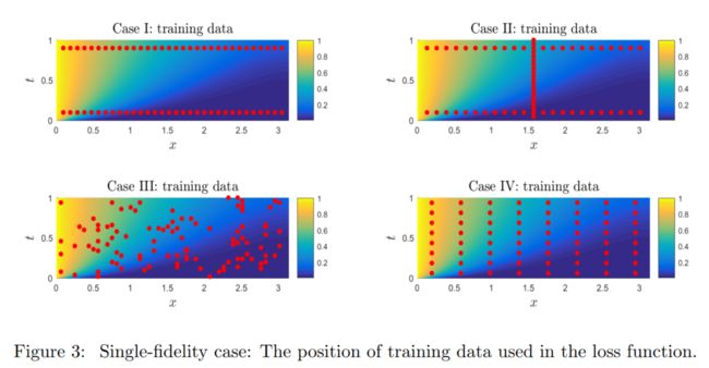
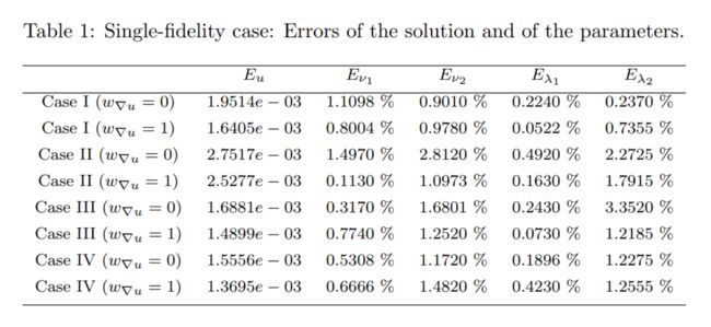
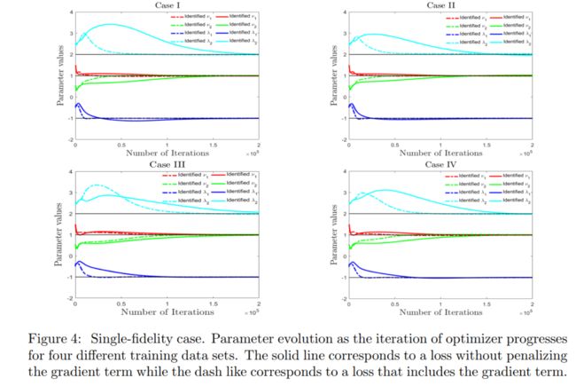
• The convergence is faster if we include the gradient penalty term$w_{{\nabla }_u}=1$

Multi-fidelity data

In many real-world applications, the training data is small and possibly inadequate to obtain even a rough estimation of the parameters.demonstrate how we can resolve this issue by resorting to supplementary data of lower fidelity that may come from cheaper instruments of lower resolution or from some computational models. We will refer to such data as \lowfidelity" and we will assume that we have a large number of such data points unlike the high-fidelity data.Here, we will employ a composite network inspired by the recent work on multi-fidelity NNs in [2].

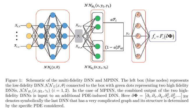
The estimator of the high-fidelity model (HF) using the correlation structure to correct the low-fidelity model (LF), can be expressed as
$$u_{HF}(x,t)=h\left(u_{LF}(x,t),x,t\right)$$
where h is a correlation map to be learned, which is based on the correlation between the HF and LF data. We have two NN for low- and highfidelity, respectively, as follows:
$$\begin{array}{rl}{u}_{LF}& =\mathcal{N}{\mathcal{N}}_{LF}\left(x_{LF},t_{LF},w_{LF},b_{LF}\right)\\ u_{HF}& =\mathcal{N}{\mathcal{N}}_{HF}\left(x_{HF},t_{HF},u_{LF},w_{HF},b_{HF}\right)\end{array}$$

Through minimizing the mean-squared-error loss function
$$MSE=MS{E}_{u_{LF}}+MS{E}_{u_{HF}}+MS{E}_{fHF}$$
where
$$\begin{array}{rl}MS{E}_{u_{LF}}& =\frac{1}{N_{LF}}\sum _{i=1}^{N_{LF}}{\left|u_{LF}\left(t_{u_{LH}}^i,x_{u_{LF}}^i\right)-u_{LH}^i\right|}^2\\ MS{E}_{u_{HF}}& =\frac{1}{N_{HF}}\sum _{i=1}^{N_{HF}}{\left|u_{HF}\left(t_{u_{HF}}^i,x_{u_{HF}}^i\right)-u_{HF}^i\right|}^2\\ MS{E}_{f_{HF}}& =\frac{1}{N_f}\sum _{i=1}^{N_f}{\left|f_{HF}\left(t_{f_{HF}}^i,x_{f_{HF}}^i\right)\right|}^2\end{array}$$

Set the true parameters
$${\nu }_1=1,{\nu }_2=1,{\lambda }_1=-1\text{ and }{\lambda }_2=2$$

• The low-fidelity training data is obtained by the second-order finite difference solution ith erroneous parameter values ${\nu }_1=1.25,{\nu }_2=1.25,{\lambda }_1=-0.75,\text{ and }{\lambda }_2=2.5$, we choose 64 point of low-fidelity, $N_{LF}=64$
• hHgh-fidelity data is obtained by the numerical solution when ${\nu }_1=1,{\nu }_2=1,{\lambda }_1=-1\text{ and }{\lambda }_2=2$, (a),$N_{HF}=12$,(b),$N_{HF}=6$
  
  

As we can see, the parameter inference using the multi-fidelity PINN is much better than the single-fidelity predictions. Moreover, if we have a small number of HF data, e.g. $N_{HF}=6$, the results of the multi-fidelity PINN are still quite accurate

Results for the stochastic case

We consider the following stochastic nonlinear ADR equation:
$$\{\begin{array}{ll}{u}_t={\left(k(x;\omega )u_x\right)}_x-{\nu }_2{u}_x+g(u)+f(x,t),& (x,t,\omega )\in \left(x_0,x_1\right)\times (0,T]\times \Omega \\ u(x,0)=1-x^2,& x\in \left(x_0,x_1\right)\\ u\left(x_0,t\right)=0,u\left(x_1,t\right)=0,& t\in (0,T]\end{array}$$
$$g(u)={\lambda }_1{u}^{{\lambda }_2}\text{ and }f(x,t)=2$$

Forward problem

Mean-squared-error loss function:
$$MSE=MS{E}_I+MS{E}_B+MS{E}_f$$
where
$$\begin{array}{rl}MS{E}_I=& \frac{1}{N\ast N_u}\sum _{s=1}^N\sum _{i=1}^{N_I}{\left[u_{NN}\left(x_u^{(i)},0;{\omega }_s\right)-u\left(x_u^{(i)},0;{\omega }_s\right)\right]}^2\\ MS{E}_B=& \frac{1}{N\ast N_B}\sum _{s=1}^N\sum _{i=1}^{N_B}{\left[u_{NN}\left(x_0,t_u^{(i)};{\omega }_s\right)-u\left(x_0,t_u^{(i)};{\omega }_s\right)\right]}^2\\ & +\frac{1}{N\ast N_B}\sum _{s=1}^N\sum _{i=1}^{N_B}{\left[u_{NN}\left(x_1,t_u^{(i)};{\omega }_s\right)-u\left(x_1,t_u^{(i)};{\omega }_s\right)\right]}^2\\ MS{E}_f=& \frac{1}{N\ast N_f}\sum _{s=1}^N\sum _{i=1}^{N_f}{\left[f_{NN}\left(x_f^{(i)},t_f^{(i)};{\omega }_s\right)-f\left(x_f^{(i)},t_f^{(i)};{\omega }_s\right)\right]}^2\end{array}$$

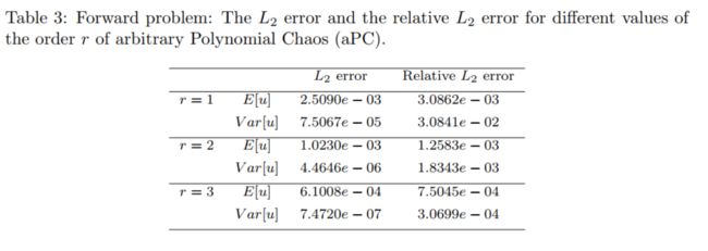
Inverse problem

we will infer the stochastic process $k(x,\omega )$ as well as the parameters
${\nu }_2,{\lambda }_1,{\lambda }_2$ and the solution $u(x,t,\omega )$

We minimize the following mean-squared-error loss function:
$$MSE=10\ast \left(MS{E}_u+MS{E}_k\right)+MS{E}_f$$

Meta-learning

We employ Bayesian Optimization (BO) to learn the optimum structure of the NNs. We use dK hidden layers and $d_K$ neurons per layer for $w_K$ mean neural network, and $d_U$hidden layers and $w_U$ neurons per layer for
ki(x); (i = 1; :::M) and uα(x; t); (α = 0; 1; ::) neural network
The target is
$$\text{Target}=10\ast \left(MS{E}_u+MS{E}_k\right)+E_{{\nu }_2}+E_{{\lambda }_1}+E_{{\lambda }_2}$$


These results suggest that we need a larger neural network for both k and u

总结：

• We addressed here a special inverse problem governed by a stochastic nonlinear advection-diffusion-reaction (ADR) equation
• We designed composite neural networks (NNs), including NNs induced by the stochastic ADR equation, and relied on spectral expansions to represent stochasticity in order to deal with the sparsity in data.
• We also presented a Bayesian Optimization method for learning the hyper-parameters of this composite NN as it is time consuming to find the proper NNs by trial and error.
  下步工作
• An important component missing in our study is quantifying the uncertaintyof the NN approximation as was first done in related work in [12] addressing the total uncertainty. This is a serious but complex issue requiring the use of multiple methods to interpret this uncertainty in an objective way, and we will pursue this line of research in future work
• one could also consider using several other methods, including genetic algorithms [19], the greedy method [20], hyperband [21, 22]as well as blended versions of the aforementioned methods or even another NN, like an RNN in conjunction with reinforcement learning [23], to search for the best architecture.

[1] M. Raissi, P. Perdikaris, G. E. Karniadakis, Physics-informed neural
networks: A deep learning framework for solving forward and inverse
problems involving nonlinear partial differential equations, Journal of
Computational Physics 378 (2019) 686{707
[2] X. Meng, G. E. Karniadakis, A composite neural network that learns
from multi-fidelity data: Application to function approximation and
inverse pde problems, arXiv preprint arXiv:1903.00104 (2019).
[3] A. M. Tartakovsky, C. O. Marrero, D. Tartakovsky, D. Barajas-Solano,
Learning parameters and constitutive relationships with physics informed deep neural networks, arXiv preprint arXiv:1808.03398 (2018).
[4] D. A. Barajas-Solano, A. M. Tartakovsky, Approximate bayesian model
inversion for pdes with heterogeneous and state-dependent coefficients,
Journal of Computational Physics (2019).
[5] M. Raissi, P. Perdikaris, G. E. Karniadakis, Numerical gaussian processes for time-dependent and nonlinear partial differential equations,
SIAM Journal on Scientific Computing 40 (2018) A172{A198.
[6] G. Pang, L. Yang, G. E. Karniadakis, Neural-net-induced gaussian process regression for function approximation and pde solution, Journal of
Computational Physics 384 (2019) 270{288.
[7] J. Han, A. Jentzen, E. Weinan, Solving high-dimensional partial differential equations using deep learning, Proceedings of the National
Academy of Sciences 115 (2018) 8505{8510.
[8] T. Q. Chen, Y. Rubanova, J. Bettencourt, D. K. Duvenaud, Neural
ordinary differential equations, in: Advances in neural information processing systems, pp. 6571{6583.
[9] P. Chaudhari, A. Oberman, S. Osher, S. Soatto, G. Carlier, Deep relaxation: partial differential equations for optimizing deep neural networks,
Research in the Mathematical Sciences 5 (2018) 30.
[10] J. Sirignano, K. Spiliopoulos, Dgm: A deep learning algorithm for solving partial differential equations, Journal of Computational Physics 375
(2018) 1339{1364.
[11] T. Qin, K. Wu, D. Xiu, Data driven governing equations approximation
using deep neural networks, Journal of Computational Physics (2019).
[12] D. Zhang, L. Lu, L. Guo, G. E. Karniadakis, Quantifying total uncertainty in physics-informed neural networks for solving forward and inverse stochastic problems, Journal of Computational Physics 397 (2019)108850.
[13] J. S. Bergstra, R. Bardenet, Y. Bengio, B. K´egl, Algorithms for hyperparameter optimization, in: Advances in neural information processing
systems, pp. 2546{2554.
[14] J. Snoek, H. Larochelle, R. P. Adams, Practical bayesian optimization
of machine learning algorithms, in: Advances in neural information
processing systems, pp. 2951{2959.
[15] J. Snoek, O. Rippel, K. Swersky, R. Kiros, N. Satish, N. Sundaram,
M. Patwary, M. Prabhat, R. Adams, Scalable bayesian optimization
using deep neural networks, in: International conference on machine
learning, pp. 2171{2180.
[16] G. Pang, L. Lu, G. E. Karniadakis, fpinns: Fractional physics-informed
neural networks, SIAM Journal on Scientific Computing 41 (2019)
A2603{A2626.
[17] X. Wan, G. E. Karniadakis, Multi-element generalized polynomial chaos
for arbitrary probability measures, SIAM Journal on Scientific Computing 28 (2006) 901{928.
[18] J. A. Paulson, E. A. Buehler, A. Mesbah, Arbitrary polynomial chaos
for uncertainty propagation of correlated random variables in dynamic
systems, IFAC-PapersOnLine 50 (2017) 3548{3553.
[19] M. Mitchell, An introduction to genetic algorithms, MIT press, 1998.
[20] Y. Li, S. Osher, Coordinate descent optimization for l1 minimization
with application to compressed sensing; a greedy algorithm, Inverse
Problems and Imaging 3 (2009) 487{503.
[21] L. Li, K. Jamieson, G. DeSalvo, A. Rostamizadeh, A. Talwalkar, Hyperband: A novel bandit-based approach to hyperparameter optimization,
Journal of Machine Learning Research 18 (2018)
[22] S. Falkner, A. Klein, F. Hutter, Bohb: Robust and efficient hyperparameter optimization at scale, arXiv preprint arXiv:1807.01774 (2018).
[23] Y. Jaafra, J. L. Laurent, A. Deruyver, M. S. Naceur, A review of metareinforcement learning for deep neural networks architecture search,
arXiv preprint arXiv:1812.07995 (2018).
[24] Y. He, J. Lin, Z. Liu, H. Wang, L.-J. Li, S. Han, Amc: Automl for
model compression and acceleration on mobile devices, in: Proceedings
of the European Conference on Computer Vision (ECCV), pp. 784{800