Zero-shot Learning 综述4

6. 直推式学习（Transductive Zero-shot Learning）

所谓直推式学习，即在ZSL中，训练模型的时候，我们可以拿到测试集的数据，只是不能拿到测试集的样本的标签，因此我们可以利用测试集数据，得到一些测试集类别的先验知识。（上文中的DMaP也是直推式学习）

典型文章：Semi-supervised Vocabulary-informed Learning (SSVoc)-2016 CVPR

当前的ZSL有以下几个缺陷：

1. ZSL 假设目标类不能分为源类（二者交集为空），反之亦然。这种问题的简化是不切实际的；（一些研究尝试用类增量的方法解决该问题）
2. 目标类的标签集合一般较小，在10到几千之间，相比之下，人能区分的类别至少30000；
3. 源类大量数据是不切实际的，因为很多类别的数据很少（目标的长尾分布）；
4. ZSL中的语义信息来源于开放的词汇集合，没有对源类的学习造成反馈。

2-4的问题暂时没有研究指出解决这些问题。而第2和3点需要大量人工代价。对于问题4，如果我们通过看图像实例来学习car这个概念，当不知道世界上还有其他的motor vehicle存在时，很可能把有4个轮子的都称为car。而truck可能与Car有更多的交集。然而，想象一下，还存在许多其他机动车辆(卡车、小型货车等)。即使没有看到这些车辆，也存在与car相关的其他知识。这足以把其他vehicle跟car区分开来，所以这时原则上应该对car的识别规则进行更新，使对car的识别更加的严谨。

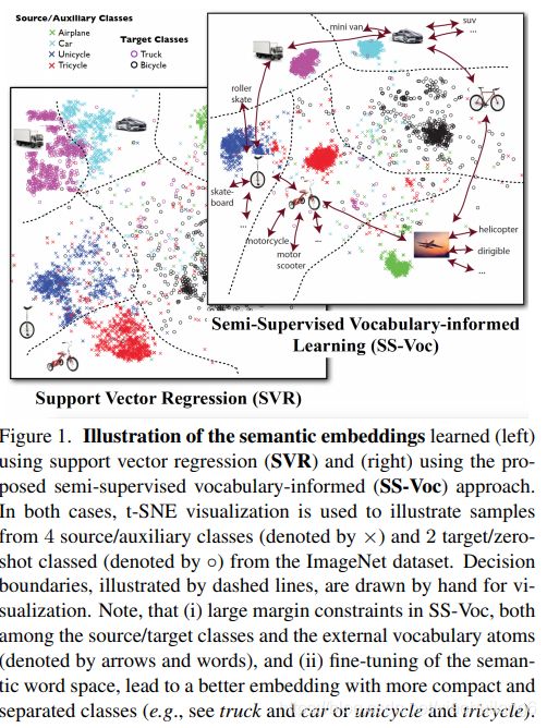
假设我们有很少标记的训练实例和一个大型开放集词汇/语义词典(以及可以学习词汇原子之间统计语义关系的文本源)，semi-supervised vocabulary-informed learning的任务是学习一个监督模型，利用语义词典帮助训练更好的分类器，以区分源类和未观察(目标)类。与其他半监督模型不同的是，该模型未标注的数据是不可用的，仅采用类别已知的数据。

模型定义：

Semi-supervised Vocabulary-informed Learning (SS-Voc)定义:  训练时利用整个词汇语义信息W进行学习，与ZSL不同的是，ZSL仅在测试时用到了测试类别的语义信息，而SS-Voc在训练时也使用了相同的语义信息。此外，SS-Voc不需要额外的数据标注或语义信息，仅仅将这些信息的利用从测试阶段迁移到训练阶段，以学习到更好的模型。

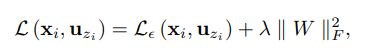
Learning Embedding

Data Term:实现上述目标的最简单方法是最小化样本投影与嵌入空间中对应原型之间的欧氏距离：

加入正则项：where || · ||F indicates the Frobenius Norm

求解方法为岭回归。为使上式的求解采用SVR，我们采用了最大间距策略- ε-−insensitive smooth SVR（ ε -SSVR）。

这种方法只解决了seen样本的嵌入问题，没有用到unseen数据的相关信息。于是文中提出了Pairwise Term的形式。

Pairwise Term:

上述数据项仅确保已标记的样本项目接近其正确的原型。然而，由于它是针对许多样本和多个类进行的，因此不太可能完全满足所有的数据约束。具体来说，如果uzi在语义空间没有其他实体 (例如, 在嵌入空间距离uzi很大),然后对xi进行映射不会导致误分类。反之，如果uzi 接近其他类别，则会导致误分类。

同理，在可见类中，也存在以下限制：

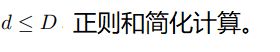
为了加速计算，与距离seen的类原型最近的unseen类原型 比较即可，即从unseen的类原型中挑了最接近seen的比较，同理，对于可见类也一样。

综上：

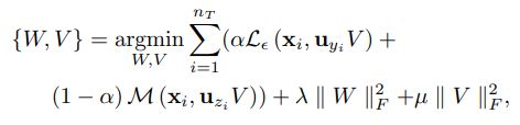
Vocabulary-informed Embedding:完整的目标函数可以表示为：

求解方法：L-BFGS

Fine-tuning Word Vector Space:假设语义空间分布均匀，线性映射是充分的，上述公式可以很好地工作。然而，我们假设词向量空间本身对于视觉判别并不一定是最优的。考虑以下情况:两个视觉上相似的类别可能出现在语义空间中很远的地方。在这种情况下，很难学习将实例与类别原型适当匹配的线性映射。因此，本文提出微调的词向量表示。优化一个全局仿射V：

Maximum Margin Embedding Recognition：

测试阶段：

采用NN进行预测。

结果：

7. 不使用额外的辅助信息

以上的模型其实都或多或少依赖于额外的辅助信息（属性、词向量等）来建立seen类和unseen类之间的迁移，于是就有人想能不能不使用额外的辅助信息来实现零次学习呢？答案是肯定的，虽然效果可能不如使用辅助信息，但是作为一种探索还是非常有意义的。

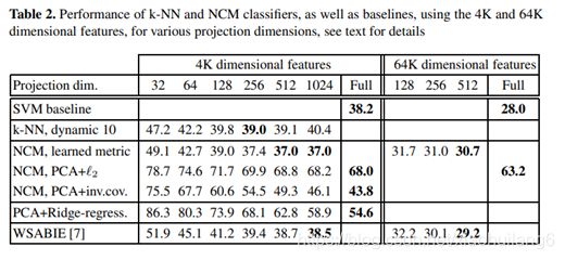
典型文章： Metric learning for large scale image classification: Generalizing to new classes at near-zero cost-2012 ECCV

借鉴了聚类和度量学习的方法，并且探索了两种方法：KNN和NCM。

它用每个类的类中心（KNN）/类均值（NCM）来取代ZSL中对于每个类的语义描述，然后学习一个度量，使得它们在seen和unseen类间共享，达到迁移的效果。

Learning Metrics to Generalize to New Categories

曼哈顿距离等效于投影后的L2距离：

Metric Learning for k-NN Classification

Query image q 和target image p（同类别）之间的距离应小于与其他类别图像n的距离。Hinge Loss：

损失函数为：

Pq 和 Nq 为Query image q 对应的正样本集和负样本集。

梯度：

LMNN中，对于query image q ，集合Pq为同类别距离q最接近的k个图像。基本原理如下:如果我们能确保这些目标比其他类的实例更接近，那么k-NN分类就会成功。然而，在实践中，对于一组给定的目标，其邻居并不总是可能实现这种情况，因为它隐式地假设原始空间中的L2距离是一个很好的相似性度量。因此，我们考虑使用一组固定的目标邻居（两种方案）：

1. 集合Pq包含与q同类别的所有图像，用同类别的损失来学习图像间相似性，相似性定义为经过学习的线性投影后图像之间的标量积；

2. Pq动态的包含k个同类别图像，最小化损失函数与Pq的选择有关。因此，根据当前的度量比原来的更接近来选择不同的目标邻居。

Metric Learning for the Nearest Class Mean Classifier

我们使用多类逻辑回归来定义NCM分类器，并定义给定图像特征向量x的类c的概率为：

其中μc为类别c的均值。我们的目标是最小化ground-truth类标签的负对数似然：

梯度：

请注意，NCM分类器在x中是线性的，因为我们将图像x赋给具有最小的距离类c*，:

结果：

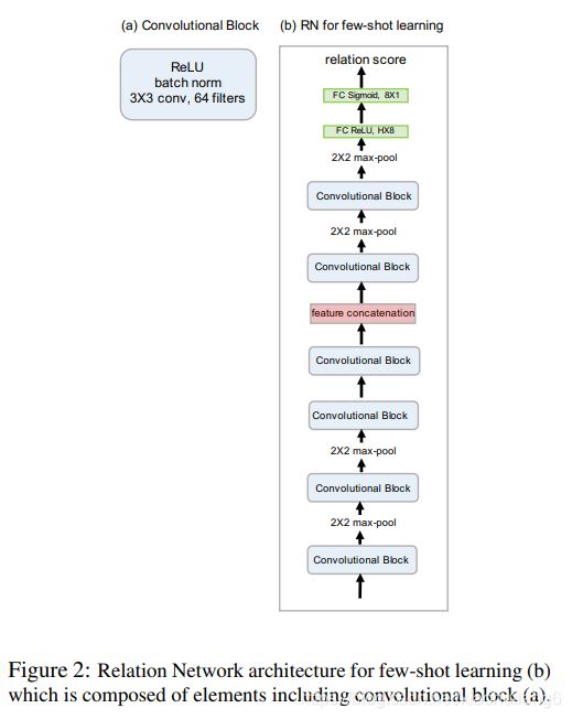
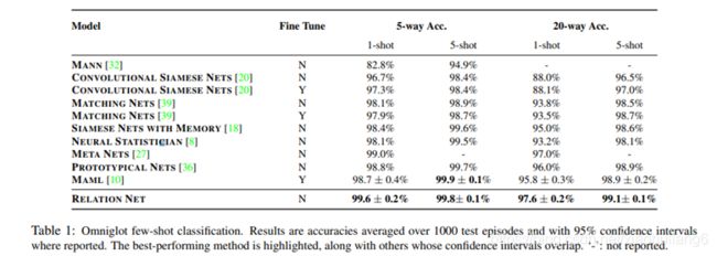
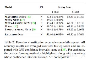
典型文章： Learning to Compare: Relation Network for Few-Shot Learning (Relation Net) – 2018 CVPR

大多数现有的few-shot learning要么需要复杂的推理机制，复杂的递归神经网络(RNN)架构，或微调目标问题。我们的方法旨在训练一个 one-shot learning的有效度量，并与其他方法高度相关。他们的重点是学习可转移嵌入和预先定义一个固定的度量(例如，如欧式距离)，我们的目标是学习一个可转移的深度度量，用于比较图像或类别之间的关系(few-shot learning)。通过更深层次解的归纳偏差表达(在嵌入和关系模块上的多个非线性学习stage)，使我们可以更容易地学习问题的求解。

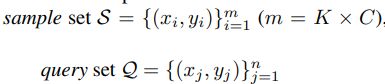
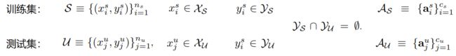
我们有三个数据集:一个训练集、一个支持集和一个测试集。支持集和测试集共享相同的标签空间，但训练集有自己的标签空间，与支持/测试集不相交。如果支持集中每个类别C包含K个样本，命名为：C-way K-shot。支持集样本较少，带标签。测试集不带标签。

利用训练集的一种有效方法是通过基于情节的训练来模拟few-shot learning。一次训练迭代中，一个情节由训练集中的随机C个类别（每个类别K个样本）组成的sample Set S和这C个类别的剩余样本部分（query set Q）组成。

上述用Q和S训练好的模型通过微调可以用于真正的支持集。

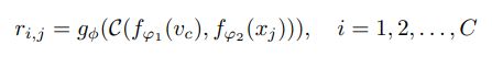
One-Shot（K=1）：如图所示

K-Shot：每个类别的样本特征求和，最终生成One-Shot。

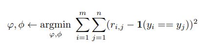
Objective function

mean square error (MSE) loss

Zero-shot Learning

支持集采用语义向量v，因此 fφ 函数对于Q和S是不同的：（严格讲，不是不使用额外的辅助信息的范畴，few-shot属于该范畴）

 Network Architecture

class AttributeNetwork(nn.Module):
    """docstring for RelationNetwork"""
    def __init__(self,input_size,hidden_size,output_size):
        super(AttributeNetwork, self).__init__()
        self.fc1 = nn.Linear(input_size,hidden_size)
        self.fc2 = nn.Linear(hidden_size,output_size)

    def forward(self,x):

        x = F.relu(self.fc1(x))
        x = F.relu(self.fc2(x))

        return x

class RelationNetwork(nn.Module):
    """docstring for RelationNetwork"""
    def __init__(self,input_size,hidden_size,):
        super(RelationNetwork, self).__init__()
        self.fc1 = nn.Linear(input_size,hidden_size)
        self.fc2 = nn.Linear(hidden_size,1)

    def forward(self,x):

        x = F.relu(self.fc1(x))
        x = F.sigmoid(self.fc2(x))
        return x
    


def main():
    # step 1: init dataset
    print("init dataset")
    
    dataroot = './data'
    dataset = 'AwA1_data'
    image_embedding = 'res101' 
    class_embedding = 'original_att'

    matcontent = sio.loadmat(dataroot + "/" + dataset + "/" + image_embedding + ".mat")
    feature = matcontent['features'].T
    label = matcontent['labels'].astype(int).squeeze() - 1
    matcontent = sio.loadmat(dataroot + "/" + dataset + "/" + class_embedding + "_splits.mat")
    # numpy array index starts from 0, matlab starts from 1
    trainval_loc = matcontent['trainval_loc'].squeeze() - 1
    test_seen_loc = matcontent['test_seen_loc'].squeeze() - 1
    test_unseen_loc = matcontent['test_unseen_loc'].squeeze() - 1
  
    attribute = matcontent['att'].T 

    x = feature[trainval_loc] # train_features
    train_label = label[trainval_loc].astype(int)  # train_label
    att = attribute[train_label] # train attributes
    
    x_test = feature[test_unseen_loc]  # test_feature
    test_label = label[test_unseen_loc].astype(int) # test_label
    x_test_seen = feature[test_seen_loc]  #test_seen_feature
    test_label_seen = label[test_seen_loc].astype(int) # test_seen_label
    test_id = np.unique(test_label)   # test_id
    att_pro = attribute[test_id]      # test_attribute
    
    
    # train set
    train_features=torch.from_numpy(x)
    print('train_features_shape: ', train_features.shape)

    train_label=torch.from_numpy(train_label).unsqueeze(1)
    print('train_label_shape: ', train_label.shape)

    # attributes
    all_attributes=np.array(attribute)
    print('all_attributes_shape: ', all_attributes.shape)
    
    attributes = torch.from_numpy(attribute)
    # test set

    test_features=torch.from_numpy(x_test)
    print('test_features_shape: ', test_features.shape)

    test_label=torch.from_numpy(test_label).unsqueeze(1)
    print('test_label_shape: ', test_label.shape)

    testclasses_id = np.array(test_id)
    print('testclasses_id_shape: ', testclasses_id.shape, 'test_classes_id: ', testclasses_id)

    test_attributes = torch.from_numpy(att_pro).float()
    print('test_attributes_shape: ', test_attributes.shape)

    
    test_seen_features = torch.from_numpy(x_test_seen)
    print('test_seen_features_shape: ', test_seen_features.shape)
    
    test_seen_label = torch.from_numpy(test_label_seen)
    
    

    train_data = TensorDataset(train_features,train_label)
    

    # init network
    print("init networks")
    attribute_network = AttributeNetwork(85,1024,2048)
    relation_network = RelationNetwork(4096,400)

    if GPU >= 0:
        attribute_network.cuda(GPU)
        relation_network.cuda(GPU)
    else:
        attribute_network.to('cpu')
        relation_network.to('cpu')

    attribute_network_optim = torch.optim.Adam(attribute_network.parameters(),lr=LEARNING_RATE,weight_decay=1e-5)
    attribute_network_scheduler = StepLR(attribute_network_optim,step_size=200000,gamma=0.5)
    relation_network_optim = torch.optim.Adam(relation_network.parameters(),lr=LEARNING_RATE)
    relation_network_scheduler = StepLR(relation_network_optim,step_size=200000,gamma=0.5)


    print("training...")
    last_accuracy = 0.0

    for episode in range(EPISODE):
        attribute_network_scheduler.step(episode)
        relation_network_scheduler.step(episode)

        train_loader = DataLoader(train_data,batch_size=BATCH_SIZE,shuffle=True)

        batch_features,batch_labels = train_loader.__iter__().next()

        sample_labels = []
        for label in batch_labels.numpy():
            if label not in sample_labels:
                sample_labels.append(label)
        # pdb.set_trace()
        
        sample_attributes = torch.Tensor([all_attributes[i] for i in sample_labels]).squeeze(1) # 17*85
        class_num = sample_attributes.shape[0]

        if GPU >= 0:
            batch_features = Variable(batch_features).cuda(GPU).float()  # 32*2048
            sample_features = attribute_network(Variable(sample_attributes).cuda(GPU)) #17*2048
        else:
            batch_features = Variable(batch_features).to('cpu').float()  # 32*2048
            sample_features = attribute_network(Variable(sample_attributes).to('cpu'))  #17*2048


        sample_features_ext = sample_features.unsqueeze(0).repeat(BATCH_SIZE,1,1) #32*17*2048
        batch_features_ext = batch_features.unsqueeze(0).repeat(class_num,1,1) #17*32*2048
        batch_features_ext = torch.transpose(batch_features_ext,0,1)#32*17*2048
        
        #print(sample_features_ext)
        #print(batch_features_ext)
        relation_pairs = torch.cat((sample_features_ext,batch_features_ext),2).view(-1,4096) # 544*4096
        # pdb.set_trace()
        relations = relation_network(relation_pairs).view(-1,class_num)#32*17
        #print(relations)

        # re-build batch_labels according to sample_labels
        sample_labels = np.array(sample_labels) #17*1
        re_batch_labels = []
        for label in batch_labels.numpy():
            index = np.argwhere(sample_labels==label)
            re_batch_labels.append(index[0][0])
        re_batch_labels = torch.LongTensor(re_batch_labels) # 记录训练数据的label在sample_label中的位置
        # pdb.set_trace()
        

        # loss
        if GPU >= 0:
            mse = nn.MSELoss().cuda(GPU)
            one_hot_labels = Variable(torch.zeros(BATCH_SIZE, class_num).scatter_(1, re_batch_labels.view(-1,1), 1)).cuda(GPU)
            loss = mse(relations,one_hot_labels)
        else:
            mse = nn.MSELoss().to('cpu')
            one_hot_labels = Variable(
                torch.zeros(BATCH_SIZE, class_num).scatter_(1, re_batch_labels.view(-1, 1), 1)).to('cpu')
            loss = mse(relations, one_hot_labels)
        # pdb.set_trace()

        # update
        attribute_network.zero_grad()
        relation_network.zero_grad()

        loss.backward()

        attribute_network_optim.step()
        relation_network_optim.step()

        if (episode+1)%100 == 0:
                print("episode:",episode+1,"   loss:",loss.data.item())

        if (episode+1)%2000 == 0:
            # test
            print("Testing...")

            def compute_accuracy(test_features,test_label,test_id,test_attributes):
                # test_features:[5685,2048], test_label:[5685, 1], test_id:[10,], test_attributes:[10, 85]
                test_data = TensorDataset(test_features,test_label)
                test_batch = 32
                test_loader = DataLoader(test_data,batch_size=test_batch,shuffle=False)
                total_rewards = 0
                # fetch attributes
                # pdb.set_trace()

                sample_labels = test_id
                sample_attributes = test_attributes
                class_num = sample_attributes.shape[0]
                test_size = test_features.shape[0]
                
                print("class num:",class_num)
                predict_labels_total = []
                re_batch_labels_total = []
                
                for batch_features,batch_labels in test_loader:

                    batch_size = batch_labels.shape[0]

                    if GPU >= 0:
                        batch_features = Variable(batch_features).cuda(GPU).float()  # 32*2048
                        sample_features = attribute_network(Variable(sample_attributes).cuda(GPU).float())#10*2048
                    else:
                        batch_features = Variable(batch_features).to('cpu').float()  # 32*1024
                        sample_features = attribute_network(Variable(sample_attributes).to('cpu').float())

                    sample_features_ext = sample_features.unsqueeze(0).repeat(batch_size,1,1)
                    batch_features_ext = batch_features.unsqueeze(0).repeat(class_num,1,1)
                    batch_features_ext = torch.transpose(batch_features_ext,0,1)

                    relation_pairs = torch.cat((sample_features_ext,batch_features_ext),2).view(-1,4096)
                    relations = relation_network(relation_pairs).view(-1,class_num)#32*10

                    # re-build batch_labels according to sample_labels

                    re_batch_labels = []
                    for label in batch_labels.numpy():
                        index = np.argwhere(sample_labels==label)
                        re_batch_labels.append(index[0][0])
                    re_batch_labels = torch.LongTensor(re_batch_labels)# 记录测试数据的label在sample_label中的位置
                    # pdb.set_trace()


                    _,predict_labels = torch.max(relations.data,1)
                    predict_labels = predict_labels.cpu().numpy()
                    re_batch_labels = re_batch_labels.cpu().numpy()
                    
                    predict_labels_total = np.append(predict_labels_total, predict_labels)
                    re_batch_labels_total = np.append(re_batch_labels_total, re_batch_labels)

                # compute averaged per class accuracy    
                predict_labels_total = np.array(predict_labels_total, dtype='int')
                re_batch_labels_total = np.array(re_batch_labels_total, dtype='int')
                unique_labels = np.unique(re_batch_labels_total)
                acc = 0
                for l in unique_labels:
                    idx = np.nonzero(re_batch_labels_total == l)[0]
                    acc += accuracy_score(re_batch_labels_total[idx], predict_labels_total[idx])
                acc = acc / unique_labels.shape[0]
                return acc
            
            zsl_accuracy = compute_accuracy(test_features,test_label,test_id,test_attributes)
            gzsl_unseen_accuracy = compute_accuracy(test_features,test_label,np.arange(50),attributes)
            gzsl_seen_accuracy = compute_accuracy(test_seen_features,test_seen_label,np.arange(50),attributes)
            
            H = 2 * gzsl_seen_accuracy * gzsl_unseen_accuracy / (gzsl_unseen_accuracy + gzsl_seen_accuracy)
            
            print('zsl:', zsl_accuracy)
            print('gzsl: seen=%.4f, unseen=%.4f, h=%.4f' % (gzsl_seen_accuracy, gzsl_unseen_accuracy, H))
            

            if zsl_accuracy > last_accuracy:

                # save networks
                torch.save(attribute_network.state_dict(),"./models/zsl_awa1_attribute_network_v33.pkl")
                torch.save(relation_network.state_dict(),"./models/zsl_awa1_relation_network_v33.pkl")

                print("save networks for episode:",episode)

                last_accuracy = zsl_accuracy

结果：

8. ZSL中的特征提取

ZSL中大多数工作都在关注Visual-Semantic 的嵌入问题，而少有工作去关注模型提取特征.

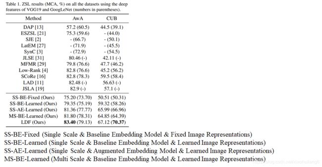
典型文章： Discriminative Learning of Latent Features for Zero-Shot Recognition (LDF) – 2018 CVPR

到目前为止，映射矩阵W的学习虽然对ZSL很重要，但主要是通过最小化视觉空间和语义空间之间的对齐损失来求解。而ZSL的主要目的是对unseen目标进行分类。因此，视觉特征和语义特征应该分开讨论。不幸的是，到目前为止，这个问题在ZSL中一直被忽视，几乎所有的方法都遵循相同的范式:1)手工制作或使用预先训练的CNN模型提取图像特征;2)利用人为设计的属性作为语义表示。这种模式存在一些缺陷：

1. 手工制作或使用预先训练的CNN模型提取的图像特征对于ZSR任务来说，不具有代表性；
2. 人工定义的语义特征并不彻底。ZSL数据集中可能存在未被预定义属性反映出来的判别性视觉特征；此外，如果两个类别(比如猎豹和老虎)共享太多(用户定义的)属性，在属性向量空间中很难区分；
3. 现有ZSL方法中的低层次特征提取和嵌入空间构建是分开处理的，通常是孤立进行的。因此，现有的工作很少在统一的框架中考虑这两个部分。

模型定义：

网络包含三个部分：FNet，ZNet，ENet

The Image Feature Network (FNet)

在ZSL中，在嵌入的同时学习图像特征。Backbone选择VGG-19或GoogleNet，特征提取表示为：

与传统的ZSL方法不同，FNet的参数是与其他部分联合训练的;因此，所获得的特征与嵌入可以很好地调节.

The Zoom Network (ZNet)

我们假设图像中的某些区别性区域对于ZSL很重要，该区域可能只包含目标本身或者局部信息。候选区域还需要反映用户定义的属性，其中一些描述了背景，如游泳、树和山。因此，期望目标区域中包含一些背景来增强属性嵌入。命名为：object-centric region。通过一个增量放大方法使网络能够自动搜索由粗到精的判别性区域。具体的，Znet的输入为Fnet的特征，为简化计算，令该区域为正方形，表示为：

zx, zy 和zs分别为正方形的中心坐标和边长。ZNet为两个级联的全连接层，并用sigmoid函数激活。获得上述信息后，通过裁剪即可得到放大区域。但是，反向传播中，裁剪是不连续的，因此，sigmoid函数首先生成一个二维连续的掩码：

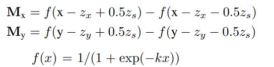
实验中k取10.裁剪操作可以表示为element-wise相乘：

裁剪后的区域通过双线性插值放缩到原始图像大小并输入到FNet。

The Embedding Network (ENet)

目标函数为：A为语义嵌入，兼容性函数得分可以用内积表示：

损失函数为：

The Augmented Embedding Model

之前的模型采用的是人工定义的属性，受size的影响，不具备判别性，我们提出了augmented attribute space, 将图像投影到人工定义的属性user-defined attributes (UA)和潜在判别属性（ discriminative attributes (LA). ）

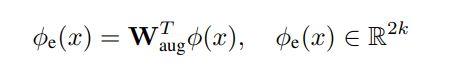
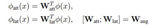
为了将嵌入特征φe(x)与UA和LA对应。我们将其分为两个部分：

前k维对应UA，后k维对应LA。前k维损失为：

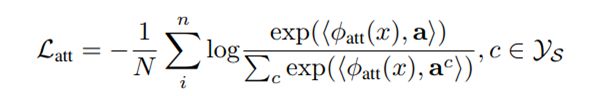
后k维损失（triplet loss）为：（xi和xk为同一类，xi和xj为不同类）

上式拆分，可得：

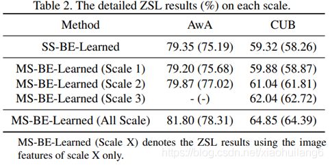
对于不同的尺度，都有softmax损失和triplet损失。对于两个尺度的网络，损失为：

Prediction：

Prediction with UA：预测函数为：

Prediction with LA：unseen类别的属性是需要的。首先对于可见类的LA属性可以求出：

对于unseen，在UA空间，类别u和类别S的关系可以求出，求解下述岭回归问题：

对于LA，

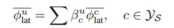
预测函数为：

Combining multiple spaces：合并上述预测

结果：

 

参考文献：

[1] Fu Y, Sigal L. Semi-supervised vocabulary-informed learning[C]//Proceedings of the IEEE Conference on Computer Vision and Pattern Recognition. 2016: 5337-5346.

[2] Mensink T, Verbeek J, Perronnin F, et al. Metric learning for large scale image classification: Generalizing to new classes at near-zero cost[M]//Computer Vision–ECCV 2012. Springer, Berlin, Heidelberg, 2012: 488-501.

[3] Sung F, Yang Y, Zhang L, et al. Learning to compare: Relation network for few-shot learning[C]//Proceedings of the IEEE Conference on Computer Vision and Pattern Recognition. 2018: 1199-1208.

[4] Li Y, Zhang J, Zhang J, et al. Discriminative learning of latent features for zero-shot recognition[C]//Proceedings of the IEEE Conference on Computer Vision and Pattern Recognition. 2018: 7463-7471.