LeGO-LOAM中的数学公式推导

LeGO-LOAM是一种在LOAM之上进行改进的激光雷达建图方法，建图效果比LOAM要好，但是建图较为稀疏，计算量也更小了。

本文原地址：wykxwyc的博客

github注释后LeGO-LOAM源码：LeGO-LOAM_NOTED
关于代码的详细理解，建议阅读：

1.地图优化代码理解

2.图像重投影代码理解

3.特征关联代码理解

4.LeGO-LOAM中的数学公式推导

以上博客会随时更新，如果对你有帮助，请点击注释代码的github仓库右上角star按钮，你的鼓励将给我更多动力。

本文 记录重新读LeGO-LOAM的代码时看到的数学运算，记录这些数学运算背后的原理，会随时更新。

featureAssociation中的数学公式

To be continued.

mapOptmization中的数学公式

cornerOptimization中的协方差矩阵计算

随机变量的协方差是什么?
1.在概率论和统计中，协方差是对两个随机变量联合分布线性相关程度的一种度量。两个随机变量越线性相关，协方差越大，完全线性无关，协方差为零。（线性无关并不代表完全无关，更不代表相互独立。）

2.两个随机变量$X$与$Y$协方差的定义如下：
$$\mathrm{cov}(X,Y)=\mathrm{E}[(X-\mathrm{E}[X])(Y-\mathrm{E}[Y])]\text{\hspace{1em}(CO-1)}$$

如何判断两个随机变量的相关程度？
1.通过定义这两个变量之间的相关系数$\eta$进行判断：
$$\eta =\frac{\mathrm{cov}(X,Y)}{\sqrt{\mathrm{var}(X)\cdot \mathrm{var}(Y)}}\text{\hspace{1em}(CO-2)}$$

1表示完全线性相关，−1表示完全线性负相关，0表示线性无关。线性无关并不代表完全无关，更不代表相互独立。

样本的协方差矩阵
1.设多维随机变量$\mathbf{X}={\left[X_1,X_2,X_3,\dots ,X_n\right]}^T$的协方差矩阵为$\Sigma$，则协方差矩阵中的每个元素为:
$${\Sigma }_{ij}=\mathrm{cov}\left(X_i,X_j\right)=\mathrm{E}\left[\left(X_i-\mathrm{E}\left[X_i\right]\right)\left(X_j-\mathrm{E}\left[X_j\right]\right)\right]\text{\hspace{1em}(CO-3)}$$
上式表示的是$X_i$和$X_j$之间的协方差。

公式CO-3也揭示了协方差矩阵中每个元素的计算过程，整个矩阵为：
$$\begin{array}{rl}& \Sigma =\mathrm{E}\left[(\mathbf{X}-\mathrm{E}[\mathbf{X}])(\mathbf{X}-\mathrm{E}[\mathbf{X}]{)}^T\right]\\ & =\left[\begin{array}{cccc}\mathrm{cov}\left(X_1,X_1\right)& \mathrm{cov}\left(X_1,X_2\right)& \dots & \mathrm{cov}\left(X_1,X_n\right)\\ \mathrm{cov}\left(X_2,X_1\right)& \mathrm{cov}\left(X_2,X_2\right)& \dots & \mathrm{cov}\left(X_2,X_n\right)\\ ⋮& ⋮& \ddots & ⋮\\ \mathrm{cov}\left(X_n,X_1\right)& \mathrm{cov}\left(X_n,X_2\right)& \cdots & \mathrm{cov}\left(X_n,X_n\right)\end{array}\right]\\ & =\left[\begin{array}{cccc}\mathrm{E}\left[\left(X_1-\mathrm{E}\left[X_1\right]\right)\left(X_1-\mathrm{E}\left[X_1\right]\right)\right]& \mathrm{E}\left[\left(X_1-\mathrm{E}\left[X_1\right]\right)\left(X_2-\mathrm{E}\left[X_2\right]\right)\right]& \cdots & \mathrm{E}\left[\left(X_1-\mathrm{E}\left[X_1\right]\right)\left(X_n-\mathrm{E}\left[X_n\right]\right)\right]\\ \mathrm{E}\left[\left(X_2-\mathrm{E}\left[X_2\right]\right)\left(X_1-\mathrm{E}\left[X_1\right]\right)\right]& \mathrm{E}\left[\left(X_2-\mathrm{E}\left[X_2\right]\right)\left(X_2-\mathrm{E}\left[X_2\right]\right)\right]& \cdots & \mathrm{E}\left[\left(X_2-\mathrm{E}\left[X_2\right]\right)\left(X_n-\mathrm{E}\left[X_n\right]\right)\right]\\ ⋮& ⋮& \ddots & ⋮\\ \mathrm{E}\left[\left(X_n-\mathrm{E}\left[X_n\right]\right)\left(X_1-\mathrm{E}\left[X_1\right]\right)\right]& \mathrm{E}\left[\left(X_n-\mathrm{E}\left[X_n\right]\right)\left(X_2-\mathrm{E}\left[X_2\right]\right)\right]& \cdots & \mathrm{E}\left[\left(X_n-\mathrm{E}\left[X_n\right]\right)\left(X_n-\mathrm{E}\left[X_n\right]\right)\right]\end{array}\right]\end{array}$$
记上面公式为(CO-4)。

2.样本的协方差矩阵的计算
样本集合为$\left\{{\mathbf{x}}_{\cdot j}={\left[x_{1j},x_{2j},\dots ,x_{nj}\right]}^T|1⩽j⩽m\right\}$，m表示样本数量。

整个样本的协方差矩阵：
$$\begin{array}{rl}& \hat{\Sigma }=\left[\begin{array}{cccc}{q}_{11}& q_{12}& \cdots & q_{1n}\\ q_{21}& q_{21}& \cdots & q_{2n}\\ ⋮& ⋮& \ddots & ⋮\\ q_{n1}& q_{n2}& \cdots & q_{nn}\end{array}\right]\\ & =\frac{1}{m-1}\left[\begin{array}{cccc}{\sum }_{j=1}^m\left(x_{1j}-{\overline{x}}_1\right)\left(x_{1j}-{\overline{x}}_1\right)& {\sum }_{j=1}^m\left(x_{1j}-{\overline{x}}_1\right)\left(x_{2j}-{\overline{x}}_2\right)& \cdots & {\sum }_{j=1}^m\left(x_{1j}-{\overline{x}}_1\right)\left(x_{nj}-{\overline{x}}_n\right)\\ {\sum }_{j=1}^m\left(x_{2j}-{\overline{x}}_2\right)\left(x_{1j}-{\overline{x}}_1\right)& {\sum }_{j=1}^m\left(x_{2j}-{\overline{x}}_2\right)\left(x_{2j}-{\overline{x}}_2\right)& \cdots & {\sum }_{j=1}^m\left(x_{2j}-{\overline{x}}_2\right)\left(x_{nj}-{\overline{x}}_n\right)\\ ⋮& ⋮& \ddots & ⋮\\ {\sum }_{j=1}^m\left(x_{nj}-{\overline{x}}_n\right)\left(x_{1j}-{\overline{x}}_1\right)& {\sum }_{j=1}^m\left(x_{nj}-{\overline{x}}_n\right)\left(x_{2j}-{\overline{x}}_2\right)& \cdots & {\sum }_{j=1}^m\left(x_{nj}-{\overline{x}}_n\right)\left(x_{nj}-{\overline{x}}_n\right)\end{array}\right]\\ & =\frac{1}{m-1}\sum _{j=1}^m\left(\mathbf{x}{.}_j-\overline{\mathbf{x}}\right){\left({\mathbf{x}}_{:j}-\overline{\mathbf{x}}\right)}^T\end{array}$$
记上面公式为CO-5。

LeGO-LOAM的代码中的协方差计算过程
1.LeGO-LOAM中的协方差采用公式OC-5中的计算方法,每个点云的维度为n=3,XYZ三个距离,一共有m=5个样本;
2.有一个区别就是代码中最后直接除以m=5，而公式OC-5中是除以m-1=4。

cornerOptimization中特征边缘的方向向量的计算

求方向向量的过程？
1.对识别为特征边缘的点计算它和它周围点的协方差矩阵，
2.然后用opencv库函数求解特征值和特征向量
3.会有一个大的特征值和两个小的特征值，大的特征值对应于方向向量。

为什么这个协方差矩阵的较大特征值对应的就是边缘的方向？
To be continued.

cornerOptimization中计算点到直线的距离

点指的是被认为是特征边缘上的点，直线就是特征边缘所在的这条直线。
简单来看就是计算点到直线的距离，用面积法进行计算。

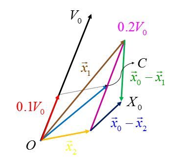
在上图中，就是求点$X_0$到紫色直线$0.2V_0$的距离。

点$X_0$对应于点pointSel，点$C$对应于点$[c_x,c_y,c_z]$，先求绿色，蓝色线段构成的平行四边形面积，然后除以紫色的长度，得到距离值。

surfOptimization中如何计算点到平面的距离

To be continued

pointAssociateToMap中对坐标变换的数学表达

这个函数中通过乘以旋转矩阵的方式，对坐标进行了变换，由局部坐标系变换到地图的全局坐标系。
变换是先进行yaw角的变换，然后是roll角的变换，最后是pitch的变换(即z->x->y),按照坐标变换左乘矩阵的规则，有：
$$p_o={\mathbf{R}}_y{\mathbf{R}}_x{\mathbf{R}}_z{p}_i+\mathbf{T}\text{\hspace{1em}(PA-1)}$$

所以整体的旋转变换可以写成一个矩阵形式：
$$\begin{gathered} {\mathbf{R}}_{total}={\mathbf{R}}_y{\mathbf{R}}_x{\mathbf{R}}_z \\ =Y_1{X}_2{Z}_3=\left[\begin{array}{ccc}{c}_1{c}_3+s_1{s}_2{s}_3& c_3{s}_1{s}_2-c_1{s}_3& c_2{s}_1\\ c_2{s}_3& c_2{c}_3& -s_2\\ c_1{s}_2{s}_3-c_3{s}_1& c_1{c}_3{s}_2+s_1{s}_3& c_1{c}_2\end{array}\right]\text{\hspace{1em}(PA-2)} \end{gathered}$$

注意：上面公式简写了$sin,cos$函数的符号。

已知roll，pitch，yaw三个角如何求得旋转矩阵？

旋转有两种，一种是向量旋转，另一张是坐标系旋转。如下图所示：

向量旋转
图R-1是向量旋转，通过平面几何公式，很容易就能得到旋转后的向量坐标是:
$${\mathbf{v}}^{\prime }={\mathbf{R}}_{\theta }{\mathbf{v}}_0=\left[\begin{array}{cc}\cos \theta & -\sin \theta \\ \sin \theta & \cos \theta \end{array}\right]\times {\mathbf{v}}_0\text{\hspace{1em}(RO-1)}$$
其中有：
$${\mathrm{R}}_{\theta }=\left[\begin{array}{cc}\cos \theta & -\sin \theta \\ \sin \theta & \cos \theta \end{array}\right]\text{\hspace{1em}(RO-2)}$$

坐标系旋转
坐标系旋转就是相当于向量的逆旋转，所以有：
$${\mathrm{R}}_{\theta }^{\prime }=\left[\begin{array}{cc}\cos \theta & \sin \theta \\ -\sin \theta & \cos \theta \end{array}\right]\text{\hspace{1em}(RO-3)}$$

三维空间中的坐标旋转
公式RO-2可以看做是绕z轴正向旋转$\theta$的角度，只有$x,y$坐标变化，$z$坐标不变，对应于yaw角的旋转，按照这种方式我们可以分别得到绕roll，pitch和yaw角的旋转公式：
$$\begin{array}{l}{\mathrm{R}}_x(\alpha )=\left[\begin{array}{ccc}1& 0& 0\\ 0& \cos \alpha & \sin \alpha \\ 0& -\sin \alpha & \cos \alpha \end{array}\right]\\ {\mathrm{R}}_y(\beta )=\left[\begin{array}{ccc}\cos \beta & 0& -\sin \beta \\ 0& 1& 0\\ \sin \beta & 0& \cos \beta \end{array}\right]\\ {\mathrm{R}}_z(\gamma )=\left[\begin{array}{ccc}\cos \gamma & \sin \gamma & 0\\ -\sin \gamma & \cos \gamma & 0\\ 0& 0& 1\end{array}\right]\end{array}\text{\hspace{1em}(RO-4)}$$
注意上式中的绕y轴的pitch旋转和另外两个有点不同。

LeGO中的坐标旋转问题
LeGO中的局部坐标系下的点转换到全局坐标系中去的过程在pointAssociateToMap中对坐标变换的数学表达中以及说明,根据公式PA-2，我们可以得到pointAssociateToMap对点进行的坐标变换：
旋转(记为公式RO-5)：
$$R=\left[\begin{array}{ccc}co{s}_{ex}co{s}_{ez}+si{n}_{ex}si{n}_{ey}si{n}_{ez}& co{s}_{ez}si{n}_{ex}si{n}_{ey}-co{s}_{ex}si{n}_{ez}& co{s}_{ey}si{n}_{ex}\\ co{s}_{ey}si{n}_{ez}& co{s}_{ey}co{s}_{ez}& -si{n}_{ey}\\ co{s}_{ex}si{n}_{ey}si{n}_{ez}-co{s}_{ez}si{n}_{ex}& co{s}_{ex}co{s}_{ez}si{n}_{ey}+si{n}_{ex}si{n}_{ez}& co{s}_{ex}co{s}_{ey}\end{array}\right]$$

平移：
$$t=\left[\begin{array}{c}{t}_x\\ t_y\\ t_z\end{array}\right]$$

LMOptimization中如何进行优化迭代计算

先明确优化函数中的优化目标
优化函数优化的量是特征点与对应直线的距离(或者特征点与特征平面的距离)。
按照最优的情况下来说，特征点应该是在特征直线（或者特征平面）上的，所以距离应该为0.

但是当特征点到直线或者平面的距离不为0的时候，说明这个点由于运动产生了畸变，我们一开始估计的旋转$R$和平移$T$估计得不准确。所以对这个旋转和平移要进行调整。也就是每次优化后进行的如下操作：

transformTobeMapped[0] += matX.at(0, 0);
transformTobeMapped[1] += matX.at(1, 0);
transformTobeMapped[2] += matX.at(2, 0);
transformTobeMapped[3] += matX.at(3, 0);
transformTobeMapped[4] += matX.at(4, 0);
transformTobeMapped[5] += matX.at(5, 0);

其中的变换涉及到对旋转矩阵求雅克比，对距离求导等。

先明确一下优化中涉及到的定义
1.局部坐标系中的点
$$X_{(k+1,i)}^L=(px,py,pz{)}^T\text{\hspace{1em}(LM-a)}$$
这里的点是特征点，边缘上的点或者平面上的点，点i在LiDAR坐标系下,k+1时刻的坐标.

2.变换$T_{(k+1)}^w$表示特征点经过这个变换内包含的3个旋转个3个平移，可以准确地变换到全局地图中，与地图中特征边缘和平面的距离为0；

3.将从局部坐标系变换到全局地图坐标系的变换定义成一个函数$G(.)$这个函数将局部点$X_{(k+1,i)}^L$转换到全局点$X_{(k+1,i)}^w$。
$$X_{(k+1,i)}^w=G\left(X_{(k+1,i)}^L,T_{(k+1)}^w\right)=R\cdot X_{(k+1,i)}^L+t\text{\hspace{1em}(LM-b)}$$

4.定义误差
$$\text{loss}=d=D\left(X_{(k+1,i)}^w,map\right)\text{\hspace{1em}(LM-c)}$$

结合公式LM-b，LM-c
$$\begin{array}{rl}& loss=d=D\left(X_{(k+1,i)}^w,map\right)\\ & =D\left(G\left(X_{(k+1,i)}^L,T_{(k+1)}^w\right),map\right)\\ & =D\left(R\cdot X_{(k+1,i)}^L+t,map\right)\end{array}\text{\hspace{1em}(LM-d)}$$

5.误差对旋转求偏导的过程

$$\begin{array}{c}\frac{\partial \mathrm{loss}}{\partial ex}=\frac{\partial D\left(G\left(X_{(k+1,i)}^L,T_{(k+1)}^w\right),map\right)}{\partial ex}\\ =\frac{\partial D(.)}{\partial G(.)}\cdot \frac{\partial G(.)}{\partial ex}\\ =\frac{\partial D(.)}{\partial G(.)}\cdot \frac{\partial \left(R\cdot X_{(k+1,1)}^L+t\right)}{\partial ex}\\ =\frac{\partial D(.)}{\partial G(.)}\cdot \frac{\partial \left(R\cdot X_{(k+1,i)}^L\right)}{\partial ex}+\frac{\partial D(.)}{\partial G(.)}\cdot \frac{\partial (t)}{\partial ex}\\ =\frac{\partial D(.)}{\partial G(.)}\cdot \frac{\partial \left(R\cdot X_{(k+1,i)}^L\right)}{\partial ex}\end{array}\text{\hspace{1em}(LM-e)}$$

6.误差对平移求偏导的过程

$$\begin{array}{c}\frac{\partial \mathrm{loss}}{\partial x}=\frac{\partial D\left(G\left(X_{(k+1,i)}^L,T_{(k+1)}^w\right),map\right)}{\partial x}\\ =\frac{\partial D(.)}{\partial G(.)}\cdot \frac{\partial G(.)}{\partial x}\\ =\frac{\partial D(.)}{\partial G(.)}\cdot \frac{\partial \left(R\cdot X_{(k+1,1)}^L+t\right)}{\partial x}\\ =\frac{\partial D(.)}{\partial G(.)}\cdot \frac{\partial \left(R\cdot X_{(k+1,i)}^L\right)}{\partial x}+\frac{\partial D(.)}{\partial G(.)}\cdot \frac{\partial (t)}{\partial x}\\ =0+\frac{\partial D(.)}{\partial G(.)}\cdot \frac{\partial (t)}{\partial x}\\ =\frac{\partial D(.)}{\partial G(.)}\end{array}\text{\hspace{1em}(LM-f)}$$

6.$\frac{\partial D(\cdot )}{\partial G(\cdot )}$的求解
$$\frac{\partial D(.)}{\partial G(.)}=\frac{\partial d}{\left(\partial X_{((k+1,i))}^w\right)}\text{\hspace{1em}(LM-g)}$$

公式LM-g中对全局坐标系中的点求导，可以理解成求一个全局点的移动方向，点在这个方向上移动，$d$减小得最快。

所以这个方向就是沿着垂线的方向。
所以点到直线的方向就是底边的垂线方向。
点到平面的方向就是平面的法线方向。

$$\frac{\partial D(.)}{\partial G(.)}=\frac{\partial d}{\left(\partial X_{((k+1,i))}^w\right)}=\left(\frac{\partial d}{\partial x},\frac{\partial d}{\partial y},\frac{\partial d}{\partial z}\right)=(la,lb,lc)$$

所以总结一下上面求解的两个部分：
$$\begin{array}{rl}& \frac{\partial \left(R\ast X_{(k+1,i)}^L\right)}{\partial ex}=\frac{\partial \left(R\right)}{\partial ex}\cdot X_{(k+1,i)}^L\\ & =\frac{\partial \left(R\right)}{\partial ex}\cdot {\left(p_x,p_y,p_z\right)}^T\\ & =\left[\begin{array}{ccc}sy\cdot cx\cdot sz& cz\cdot sy\cdot cx& -sx\cdot sy\\ -sx\cdot sz& -sx\cdot cz& -cx\\ cy\cdot cx\cdot sz& cy\cdot cz\cdot cx& -cy\cdot sx\end{array}\right]\cdot {\left(p_x,p_y,p_z\right)}^T\end{array}\text{\hspace{1em}(LM-h)}$$

同样的做法可以求得
$$\frac{\partial \left(R\times X_{(k+1,i)}^L\right)}{\partial ey}$$
以及
$$\frac{\partial \left(R\times X_{(k+1,i)}^L\right)}{\partial ez}$$
,分别对应于代码中的ary和arz。

迭代计算的过程
代码中用的是高斯-牛顿法进行迭代计算求解的。
高斯-牛顿法的基本形式为：
$$J^{T}J\Delta x=-J\cdot f(x)$$

代码中，雅克比矩阵$J$为matA,
$$matA=\left[\begin{array}{c}\frac{\partial d}{\partial roll}\\ \frac{\partial d}{\partial pitch}\\ \frac{\partial d}{\partial yaw}\\ \frac{\partial d}{\partial t_x}\\ \frac{\partial d}{\partial t_y}\\ \frac{\partial d}{\partial t_z}\end{array}\right]\text{\hspace{1em}(matA)}$$

transformFusion中的数学公式

To be continued.

参考文献及链接

1.苦力笨笨的博客:https://www.cnblogs.com/terencezhou/p/6235974.html
2.知乎SLAM专栏-「能儿」的回答：https://zhuanlan.zhihu.com/p/57351961
3.mathworld.wolfram.com：http://mathworld.wolfram.com/RotationMatrix.html
4.维基百科旋转矩阵解释：https://en.wikipedia.org/wiki/Euler_angles#Definition_by_intrinsic_rotations