Build a Credit Scoring Card Model with Python

Build a Credit Scoring Card Model with Python

1. Background Introduction

The credit scorecard model has been widely used in the field of credit risk assessment and financial risk control. The principle is to discretize the model variable WOE encoding method and then use the logistic regression model to perform a generalized linear model of the two categorical variables.

This paper will provide reference for risk control of financial lending institutions, including data preprocessing, feature variable selection, variable WOE coding discretization, logistic regression model development evaluation, credit scorecard and automatic scoring system creation.。

2. Data Description

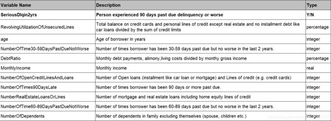
The data comes from Kaggle’s Give Me Some Credit competition, where the cs-training.csv file has 150,000 sample data and contains 11 variables, as shown in the table below.

3. Import Data

3.1. read data

import numpy as np
import pandas as pd
data=pd.read_csv('cs-training.csv')
data=data.iloc[:,1:]
data.head()

3.2. overview data

data.shape

(150000, 11)

data.describe()

data.info()

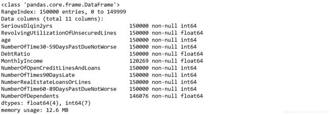
It can be seen from the results that the feature quantity MonthlyIncome is missing a large number of 29,731; while the NumberOfDependts is missing a small number of 3,924.

4. Data Preprocessing

4.1. Missing Value Processing

Data loss is very common in real-world problems, which leads to some analysis methods that cannot handle missing values. Therefore, the first step in the development of credit risk rating model requires missing value processing.

Methods for missing value processing include the following:
(1) Directly delete samples with missing values.
(2) Fill in the missing values based on the similarity between the samples.
(3) Fill in the missing values based on the correlation between the variables.

The missing rate of the variable MonthlyIncome is relatively large, so we fill in the missing values according to the correlation between the variables and fill them with the random forest method.

from sklearn.ensemble import RandomForestRegressor
def add_missing(df):
    process_df=df.ix[:,[5,0,1,2,3,4,6,7,8,9]]
    #Divided into two parts: known feature values and position feature values
    known=process_df[process_df['MonthlyIncome'].notnull()].as_matrix()
    unknown=process_df[process_df['MonthlyIncome'].isnull()].as_matrix()
    Y=known[:,0]
    X=known[:,1:]
    rfr=RandomForestRegressor(random_state=0,n_estimators=200,max_depth=3,n_jobs=-1)
    rfr.fit(X,Y)
    predicted=rfr.predict(unknown[:,1:])
    df.loc[df['MonthlyIncome'].isnull(),'MonthlyIncome']=predicted
    return df
ta=add_missing(data)

The NumberOfDependents variable has fewer missing values and can be deleted directly without affecting the overall model. In addition, after the missing values are processed, the duplicates should be deleted.

data=data.dropna()
data=data.drop_duplicates()

4.2. Outlier Processing

Outliers are values that deviate significantly from most sampled data. For example, when an individual’s age is greater than 100 or less than 0, the value is generally considered to be an outlier. , We usually use outlier detection to find outliers in the sample population. Outlier detection methods include univariate outlier detection, local outlier detection, and outlier detection based on clustering.

In this data set, univariate outlier detection is used to determine outliers, and a box plot is used. For the age variable, we think that it is an abnormal value greater than 100 years old and less than or equal to 0 years old. It can be seen from the box plot that there are not many abnormal value samples, so we can delete it directly.

import matplotlib.pyplot as plt
%matplotlib inline
dataage=data[['age']]
dataage.boxplot()

data_box = data.iloc[:,[3]]
data_box.boxplot()

data_box = data.iloc[:,[7]]
data_box.boxplot()

data_box = data.iloc[:,[9]]
data_box.boxplot()

As we can see from the above four figures, four variables including age, NumberOfTime30-59, NumberOfTimes90, and NumberOfTime60-89 all have abnormal values. If we excluding the 96, 98 values of one of these three variables, the other variables will be removed accordingly.

The good customer in the data set is 0, and the default customer is 1. Considering the normal understanding, the customer who can perform the contract and pay interest is 1 and negated.

data=data[data['age']>0]
data=data[data['NumberOfTimes90DaysLate']<90]
data['SeriousDlqin2yrs']=1-data['SeriousDlqin2yrs']

4.3. Data Segmentation

In order to verify the fitting effect of the model, we need to segment the data set into a training set and a test set.

from sklearn.cross_validation import train_test_split
Y=data['SeriousDlqin2yrs']
X=data.ix[:,1:]
X_train,X_test,Y_train,Y_test=train_test_split(X,Y,test_size=0.3,random_state=0)
train=pd.concat([Y_train,X_train],axis=1)
test=pd.concat([Y_test,X_test],axis=1)
train.to_csv('TrainData.csv',index=False)
test.to_csv('TestData.csv',index=False)

4.4. Exploratory Data Analysis

Before building a model, we typically perform Exploratory Data Analysis on existing data. EDA refers to the exploration of existing data (especially the original data obtained from surveys or observations) with as few a priori assumptions as possible. Commonly used exploratory data analysis methods are: histogram, scatter plot and box plot. For example, we analyze the feature age and monthly income as follows.

import seaborn as sns
age=data['age']
sns.distplot(age)

The distribution of age is roughly normal, consistent with statistical analysis assumptions.

mi=data[data['MonthlyIncome']<50000]['MonthlyIncome']
sns.distplot(mi)

In order to make the graphics more intuitive, set the x-axis range to less than 50,000. The distribution of monthly income is roughly normal distribution, in line with statistical analysis assumptions.

This kind of chart analysis can also be done for other variables.

5. Variable Selection

Feature variable selection (sorting) is very important for data analysis and machine learning practitioners. Good feature selection can improve the performance of the model, and help us understand the characteristics of the data and the underlying structure. This will play an important role in further improving the model and algorithm. In this paper, we use the variable selection method of the credit scoring model to determine whether the indicator is economically meaningful through the WOE analysis method, that is, by comparing the default probability of the indicator bin and the corresponding bin.

First we discretize the variables (binning).

5.1. Variable Binning

Discretization of continuous variables—there commonly uses equidistant segments, equal-depth segments, and optimal segments in the development of credit scorecards. Firstly, the optimal segmentation of continuous variables is selected. When the distribution of continuous variables does not meet the requirements of optimal segmentation, then the continuous variables are equally segmented.

The code for the optimal bin is as follows:

import scipy.stats as stats
def mono_bin(Y,X,n):
    good=Y.sum()
    bad=Y.count()-good
    r=0
    while np.abs(r)<1:
        d1=pd.DataFrame({'X':X,'Y':Y,'Bucket':pd.qcut(X,n)})
        d2=d1.groupby(['Bucket'])
        r,p=stats.spearmanr(d2['X'].mean(),d2['Y'].mean())
        n=n-1
    print(r,n)
    d3=pd.DataFrame(d2['X'].min(),columns=['min'])
    d3['min']=d2['X'].min()
    d3['max']=d2['X'].max()
    d3['sum']=d2['Y'].sum()
    d3['total']=d2['Y'].count()
    d3['rate']=d2['Y'].mean()
    d3['goodattribute']=d3['sum']/good
    d3['badattribute']=(d3['total']-d3['sum'])/bad
    d3['woe']=np.log(d3['goodattribute']/d3['badattribute'])
    iv=((d3['goodattribute']-d3['badattribute'])*d3['woe']).sum()
    d4=d3.sort_index(by='min')
    woe=list(d4['woe'].values)
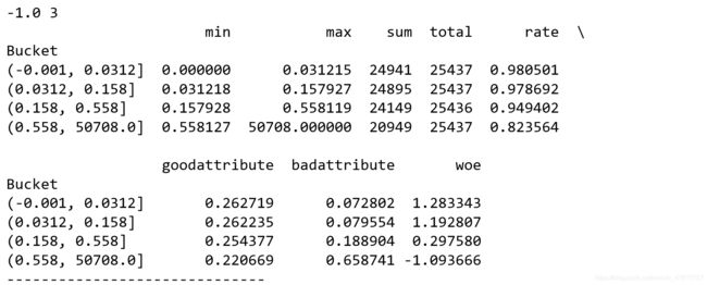
    print(d4)
    print('-'*30)
    cut=[]
    cut.append(float('-inf'))
    for i in range(1,n+1):
        qua=X.quantile(i/(n+1))
        cut.append(round(qua,4))
    cut.append(float('inf'))
    return d4,iv,woe,cut
dfx1,ivx1,woex1,cutx1=mono_bin(train['SeriousDlqin2yrs'],train['RevolvingUtilizationOfUnsecuredLines'],n=10)
dfx2, ivx2,woex2,cutx2=mono_bin(train['SeriousDlqin2yrs'], train['age'], n=10)
dfx4, ivx4,woex4,cutx4 =mono_bin(train['SeriousDlqin2yrs'],train['DebtRatio'], n=20)
dfx5, ivx5,woex5,cutx5=mono_bin(train['SeriousDlqin2yrs'], train['MonthlyIncome'], n=10)    

For variables that are not optimally binned, the bins are as follows:

def self_bin(X,Y,cat):
    good=Y.sum()
    bad=Y.count()-good
    d1=pd.DataFrame({'X':X,'Y':Y,'Bucket':pd.cut(X,cat)})
    d2=d1.groupby(['Bucket'])
    d3=pd.DataFrame(d2['X'].min(),columns=['min'])
    d3['min']=d2['X'].min()
    d3['max']=d2['X'].max()
    d3['sum']=d2['Y'].sum()
    d3['total']=d2['Y'].count()
    d3['rate']=d2['Y'].mean()
    d3['goodattribute']=d3['sum']/good
    d3['badattribute']=(d3['total']-d3['sum'])/bad
    d3['woe']=np.log(d3['goodattribute']/d3['badattribute'])
    iv=((d3['goodattribute']-d3['badattribute'])*d3['woe']).sum()
    d4=d3.sort_index(by='min')
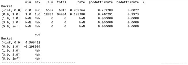
    print(d4)
    print('-'*40)
    woe=list(d3['woe'].values)
    return d4,iv,woe
ninf = float('-inf')
pinf = float('inf')
cutx3 = [ninf,0,1,3,5,pinf]
cutx6 = [ninf, 1, 2, 3, 5, pinf]
cutx7 = [ninf, 0, 1, 3, 5, pinf]
cutx8 = [ninf, 0,1,2, 3, pinf]
cutx9 = [ninf, 0, 1, 3, pinf]
cutx10 = [ninf, 0, 1, 2, 3, 5, pinf]
dfx3,ivx3,woex3=self_bin(train['SeriousDlqin2yrs'],train['NumberOfTime30-59DaysPastDueNotWorse'],cutx3)
dfx6, ivx6 ,woex6= self_bin(train['SeriousDlqin2yrs'], train['NumberOfOpenCreditLinesAndLoans'], cutx6)
dfx7, ivx7,woex7 = self_bin(train['SeriousDlqin2yrs'], train['NumberOfTimes90DaysLate'], cutx7)
dfx8, ivx8,woex8 = self_bin(train['SeriousDlqin2yrs'], train['NumberRealEstateLoansOrLines'], cutx8)
dfx9, ivx9,woex9 = self_bin(train['SeriousDlqin2yrs'], train['NumberOfTime60-89DaysPastDueNotWorse'], cutx9)
dfx10, ivx10,woex10 = self_bin(train['SeriousDlqin2yrs'], train['NumberOfDependents'], cutx10)

5.2. WOE

The full name of WOE is “Weight of Evidence”, which is the weight of evidence. The WoE analysis is to bin the indicator, calculate the WoE value of each gear position and observe the trend of the WoE value as a function of the indicator.

The mathematical definition of WoE is: woe=ln(goodattribute/badattribute). The goodattribute calculation method is the number of good customers in each box / the total number of good customers in the data set; badattribute is calculated as the number of bad customers in each box / the total number of bad customers in the data set.

Different characteristics, after the optimal binning, different number of boxes are generated, and each interval corresponds to a woe value. The last woex1 is the woe in the list with the x1 feature.

5.3. IV Strainer

The IV of the feature is a value, and its formula is: IV=sum((goodattribute-badattribute)*woe), the full name of the IV is Infomation Value, which is generally used to compare the predictive ability of the feature. IV0.1 above has predictive ability, and above 0.2 is more predictive. Generate an IV diagram with the following code:

import matplotlib.pyplot as plt
%matplotlib inline
ivall=pd.Series([ivx1,ivx2,ivx3,ivx4,ivx5,ivx6,ivx7,ivx8,ivx9,ivx10],index=['x1','x2','x3','x4','x5','x6','x7','x8','x9','x10'])
fig=plt.figure()
ax1=fig.add_subplot(111)
ivall.plot(kind='bar',ax=ax1)
plt.show()

As can be seen from the above figure, the DebtRatio, MonthlyIncome, NumberOfOpenCreditLinesAndLoans, NumberRealEstateLoansOrLines, and NumberOfDependents variables have significantly lower IV values and poor prediction capabilities, so they are deleted.

5.4. Variable Correlation Analysis

Check the correlation between the variables with the cleaned data. Note that the correlation analysis here is only a preliminary check, and the WOE of the model (evidence weight) is further examined as the basis for the variable screening. We use the seaborn package in Python to call the heatmap() drawing function to draw. The implementation code is as follows:

import seaborn as sns
corr=data.corr()
xticks=['x0','x1','x2','x3','x4','x5','x6','x7','x8','x9','x10']
fig=plt.figure()
fig.set_size_inches(16,6)
ax1=fig.add_subplot(111)
sns.heatmap(corr,vmin=-1,vmax=1,cmap='hsv',annot=True,square=True)
ax1.set_xticklabels(xticks,rotation=0)
plt.show()

As can be seen from the above figure:
(1) The correlation between variables is very small, and there is no multicollinearity problem. If there is multiple collinearity, there may be two variables that are highly correlated and need to be reduced or eliminated.
(2) It can be seen that the three characteristics of NumberOfTime30-59DaysPastDueNotWorse, NumberOfTimes90DaysLate and NumberOfTime60-89DaysPastDueNotWorse have strong correlation with the value of SeriousDlqin2yrs (dependent variable) we want to predict.

6. Model Analysis

The Weight of Evidence (WOE) transformation can transform the Logistic regression model into a standard scorecard format. Before building the model, we need to convert the filtered variables to WoE values for credit scoring.

6.1. Woe Conversion

We have been able to get the binned data and woe data for each variable, only need to be replaced according to the variable data, the implementation code is as follows:

data=pd.read_csv('TrainData.csv')
from pandas import Series
def replace_woe(series,cut,woe):
    list=[]
    i=0
    while i < len(series):
        valuek=series[i]
        j=len(cut)-2
        m=len(cut)-2
        while j>=0:
            if valuek<=cut[j]:
                j=-1
            else:
                j-=1
                m-=1
        list.append(woe[m])
        i+=1
    return list
data['RevolvingUtilizationOfUnsecuredLines'] = Series(replace_woe(data['RevolvingUtilizationOfUnsecuredLines'], cutx1, woex1))
data['age'] = Series(replace_woe(data['age'], cutx2, woex2))
data['NumberOfTime30-59DaysPastDueNotWorse'] = Series(replace_woe(data['NumberOfTime30-59DaysPastDueNotWorse'], cutx3, woex3))
data['DebtRatio'] = Series(replace_woe(data['DebtRatio'], cutx4, woex4))
data['MonthlyIncome'] = Series(replace_woe(data['MonthlyIncome'], cutx5, woex5))
data['NumberOfOpenCreditLinesAndLoans'] = Series(replace_woe(data['NumberOfOpenCreditLinesAndLoans'], cutx6, woex6))
data['NumberOfTimes90DaysLate'] = Series(replace_woe(data['NumberOfTimes90DaysLate'], cutx7, woex7))
data['NumberRealEstateLoansOrLines'] = Series(replace_woe(data['NumberRealEstateLoansOrLines'], cutx8, woex8))
data['NumberOfTime60-89DaysPastDueNotWorse'] = Series(replace_woe(data['NumberOfTime60-89DaysPastDueNotWorse'], cutx9, woex9))
data['NumberOfDependents'] = Series(replace_woe(data['NumberOfDependents'], cutx10, woex10))

test= pd.read_csv('TestDate.csv')
test['RevolvingUtilizationOfUnsecuredLines'] = Series(replace_woe(test['RevolvingUtilizationOfUnsecuredLines'], cutx1, woex1))
test['age'] = Series(replace_woe(test['age'], cutx2, woex2))
test['NumberOfTime30-59DaysPastDueNotWorse'] = Series(replace_woe(test['NumberOfTime30-59DaysPastDueNotWorse'], cutx3, woex3))
test['DebtRatio'] = Series(replace_woe(test['DebtRatio'], cutx4, woex4))
test['MonthlyIncome'] = Series(replace_woe(test['MonthlyIncome'], cutx5, woex5))
test['NumberOfOpenCreditLinesAndLoans'] = Series(replace_woe(test['NumberOfOpenCreditLinesAndLoans'], cutx6, woex6))
test['NumberOfTimes90DaysLate'] = Series(replace_woe(test['NumberOfTimes90DaysLate'], cutx7, woex7))
test['NumberRealEstateLoansOrLines'] = Series(replace_woe(test['NumberRealEstateLoansOrLines'], cutx8, woex8))
test['NumberOfTime60-89DaysPastDueNotWorse'] = Series(replace_woe(test['NumberOfTime60-89DaysPastDueNotWorse'], cutx9, woex9))
test['NumberOfDependents'] = Series(replace_woe(test['NumberOfDependents'], cutx10, woex10))

6.2. Logistic Model Building

import statsmodels.api as sm
Y=data['SeriousDlqin2yrs']
X=data.drop(['SeriousDlqin2yrs','DebtRatio','MonthlyIncome', 'NumberOfOpenCreditLinesAndLoans','NumberRealEstateLoansOrLines','NumberOfDependents'],axis=1)
X1=sm.add_constant(X)
logit=sm.Logit(Y,X1)
result=logit.fit()
print(result.summary2())

Assuming that the significance level is set to 0.01, as can be seen from the above figure, the logistic regression variables have passed the significance test to meet the requirements.

6.3. Model Verification

To verify the predictive power of this model, we evaluate the fit of the model through the ROC curve and AUC.

from sklearn.metrics import roc_curve,auc
import matplotlib
matplotlib.rcParams['font.sans-serif'] = ['FangSong']  
matplotlib.rcParams['axes.unicode_minus'] = False
Y_test=test['SeriousDlqin2yrs']
X_test=test.drop(['SeriousDlqin2yrs','DebtRatio','MonthlyIncome', 'NumberOfOpenCreditLinesAndLoans','NumberRealEstateLoansOrLines','NumberOfDependents'],axis=1)

X2=sm.add_constant(X_test)
resu=result.predict(X2)
fpr,tpr,threshold=roc_curve(Y_test,resu)

rocauc=auc(fpr,tpr)
plt.plot(fpr,tpr,'b',label='AUC=%0.2f'% rocauc)
plt.legend(loc='lower right')
plt.plot([0,1],[0,1],'r--')
plt.xlabel('False Positive Rate')
plt.ylabel('True Positive Rate')
plt.show()

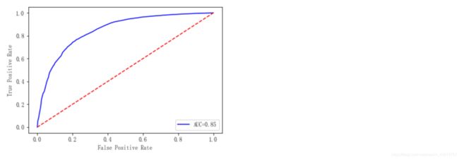
As can be seen from the above figure, the AUC value is 0.85, indicating that the prediction ability of the model is better and the correct rate is higher. It is proved that using the current five characteristics, it is effective to form a part of the score of the credit score card, and the prediction ability is better.

7. Credit Scoring Card Construction

Convert the Logistic model to the form of a standard scoring card.

Before setting up a standard scoring card, we need to select several scoring card parameters: base score, PDO (the score doubled), and the good/worst ratio. We take 600 points for the base score, PDO is 20 (the ratio is 20 times for every 20 points), and the ratio is 20 for good or bad.

Total personal score = base score + score for each part

def get_score(coe,woe,p):
    scores=[]
    for w in woe:
        score=round(coe*w*p,0)
        scores.append(score)
    return scores

def compute_score(series,cut,scores):
    i=0
    list=[]
    while i=0:
            if value>=cut[j]:
                j=-1
            else:
                j=j-1
                m=m-1
        list.append(scores[m])
        i=i+1  
    return list

coe=[9.738849,0.638002,0.505995,1.032246,1.790041,1.131956]    
import math
p = 20 / math.log(2)     
q = 600 - 20 * math.log(20) / math.log(2)    
basescore = round(q + p * coe[0], 0)

x1 = get_score(coe[1], woex1, p)
x2 = get_score(coe[2], woex2, p)
x3 = get_score(coe[3], woex3, p)
x7 = get_score(coe[4], woex7, p)
x9 = get_score(coe[5], woex9, p)

print(x1)
print(x2)
print(x3)
print(x7)
print(x9)
test1=pd.read_csv('TestData.csv')

test1['BaseScore']=Series(np.zeros(len(test1))+basescore)
test1['x1']=Series(compute_score(test1['RevolvingUtilizationOfUnsecuredLines'],cutx1,x1))
test1['x2'] = Series(compute_score(test1['age'], cutx2, x2))
test1['x3'] = Series(compute_score(test1['NumberOfTime30-59DaysPastDueNotWorse'], cutx3, x3))
test1['x7'] = Series(compute_score(test1['NumberOfTimes90DaysLate'], cutx7, x7))
test1['x9'] = Series(compute_score(test1['NumberOfTime60-89DaysPastDueNotWorse'], cutx9, x9))
test1['score']= test1['BaseScore']+test1['x1']+test1['x2']+test1['x3']+test1['x7']+test1['x9']
test1.to_csv('scoredata.csv')

test1.loc[:,['SeriousDlqin2yrs','BaseScore', 'x1', 'x2', 'x3', 'x7', 'x9', 'score']].head()

This paper uses the random forest algorithm to fit the missing values by using data on the Kaggle, the combination of the credit scorecard and the data preprocessing, variable selection, modeling analysis and prediction. The pandas package cleans up the data and visualizes the data using matplotlib, seaborn drawing packages, and uses a logistic regression model. Finally, a simple credit scoring system is created using some of the features verified by the model.

7. References

7.1. Modeling Analysis of Credit Score Card Based on Python——CSDN