Layer/Batch/Instance Normalization
总览
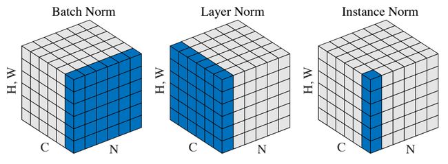
图中N表示batch,C表示CV中的通道(NLP中的序列长度、时间步),如果是图像则【H,W】表示每个通道下二维像素矩阵的高和宽,NLP中就只有一维特征向量。Batch Norm依赖Batch,对【Batch, H, W】三个维度做标准化;Layer Norm不依赖Batch,对【C,H,W】三个维度做标准化。Instance Norm既不受Batch也不受其它通道的影响,只对【H,W】两个维度做标准化。
三种标准化的表示式形式都相同,其区别在于 x x x的表示不同,其公式如下:
y = x − E [ x ] Var [ x ] + ϵ ∗ γ + β y=\frac{x-\mathrm{E}[x]}{\sqrt{\operatorname{Var}[x]+\epsilon}} * \gamma+\beta y=Var[x]+ϵx−E[x]∗γ+β
其中,对于不同Norm方法 x x x不同, E [ x ] \mathrm{E}[x] E[x]表示期望(均值), Var [ x ] \operatorname{Var}[x] Var[x]表示方差, γ \gamma γ和 β \beta β表示可学习参数,向量大小和输入维度一致。
Batch Norm
y t i l m = x t i l m − μ i σ i 2 + ϵ ∗ γ + β , μ i = 1 H W T ∑ t = 1 T ∑ l = 1 W ∑ m = 1 H x t i l m , σ i 2 = 1 H W T ∑ t = 1 T ∑ l = 1 W ∑ m = 1 H ( x t i l m − u i ) 2 y_{t i l m}=\frac{x_{t i l m}-\mu_{i}}{\sqrt{\sigma_{i}^{2}+\epsilon}}* \gamma+\beta, \quad \mu_{i}=\frac{1}{H W T} \sum_{t=1}^{T} \sum_{l=1}^{W} \sum_{m=1}^{H} x_{t i l m}, \quad \sigma_{i}^{2}=\frac{1}{H W T} \sum_{t=1}^{T} \sum_{l=1}^{W} \sum_{m=1}^{H}\left(x_{t i l m}- u_{i}\right)^{2} ytilm=σi2+ϵxtilm−μi∗γ+β,μi=HWT1t=1∑Tl=1∑Wm=1∑Hxtilm,σi2=HWT1t=1∑Tl=1∑Wm=1∑H(xtilm−ui)2
Layer Norm
-
针对4维输入:
y t i l m = x t i l m − μ t σ t 2 + ϵ ∗ γ + β , μ t = 1 H W C ∑ i = 1 C ∑ l = 1 W ∑ m = 1 H x t i l m , σ t 2 = 1 H W C ∑ i = 1 C ∑ l = 1 W ∑ m = 1 H ( x t i l m − u t ) 2 y_{t i l m}=\frac{x_{t i l m}-\mu_{t}}{\sqrt{\sigma_{t}^{2}+\epsilon}}* \gamma+\beta, \quad \mu_{t}=\frac{1}{H W C} \sum_{i=1}^{C} \sum_{l=1}^{W} \sum_{m=1}^{H} x_{t i l m}, \quad \sigma_{t}^{2}=\frac{1}{H W C} \sum_{i=1}^{C} \sum_{l=1}^{W} \sum_{m=1}^{H}\left(x_{t i l m}- u_{t}\right)^{2} ytilm=σt2+ϵxtilm−μt∗γ+β,μt=HWC1i=1∑Cl=1∑Wm=1∑Hxtilm,σt2=HWC1i=1∑Cl=1∑Wm=1∑H(xtilm−ut)2 -
针对3维输入:
y t i l = x t i l − μ t σ t 2 + ϵ ∗ γ + β , μ t = 1 N S ∑ i = 1 S ∑ l = 1 N x t i l , σ t 2 = 1 N S ∑ i = 1 S ∑ l = 1 N ( x t i l − u t ) 2 y_{t i l}=\frac{x_{t i l}-\mu_{t}}{\sqrt{\sigma_{t}^{2}+\epsilon}}* \gamma+\beta, \quad \mu_{t}=\frac{1}{N S} \sum_{i=1}^{S} \sum_{l=1}^{N} x_{t i l}, \quad \sigma_{t}^{2}=\frac{1}{N S} \sum_{i=1}^{S} \sum_{l=1}^{N} \left(x_{t i l}- u_{t}\right)^{2} ytil=σt2+ϵxtil−μt∗γ+β,μt=NS1i=1∑Sl=1∑Nxtil,σt2=NS1i=1∑Sl=1∑N(xtil−ut)2 -
3维输入的代码测试样例:
import torch
from torch import nn

class LayerNorm(nn.Module):
    def __init__(self, features, eps=1e-5):
        super(LayerNorm, self).__init__()
        self.a_2 = nn.Parameter(torch.ones(features))
        self.b_2 = nn.Parameter(torch.zeros(features))
        self.eps = eps

    def forward(self, x):
        sizes = x.size()
        mean = x.view(sizes[0], -1).mean(-1, keepdim=True)
        std = x.view(sizes[0], -1).std(-1, keepdim=True)
        mean = torch.repeat_interleave(mean, repeats=9, dim=1).view(2, 3, 3)
        std = torch.repeat_interleave(std, repeats=9, dim=1).view(2, 3, 3)
        return self.a_2 * (x - mean) / (std + self.eps) + self.b_2

norm_2 = LayerNorm(features=[2, 3, 3])
norm = nn.LayerNorm(normalized_shape=(3, 3), elementwise_affine=True)
a = torch.tensor([[[1, 2, 3],
                   [4, 5, 6],
                   [7, 8, 9]],
                  [[4, 5, 6],
                   [7, 8, 9],
                   [10, 11, 12]]], dtype=torch.float32)

print(norm(a))
print(norm_2(a))
- 代码运行结果:
tensor([[[-1.5492, -1.1619, -0.7746],
         [-0.3873,  0.0000,  0.3873],
         [ 0.7746,  1.1619,  1.5492]],

        [[-1.5492, -1.1619, -0.7746],
         [-0.3873,  0.0000,  0.3873],
         [ 0.7746,  1.1619,  1.5492]]], grad_fn=<NativeLayerNormBackward>)
tensor([[[-1.4606, -1.0954, -0.7303],
         [-0.3651,  0.0000,  0.3651],
         [ 0.7303,  1.0954,  1.4606]],

        [[-1.4606, -1.0954, -0.7303],
         [-0.3651,  0.0000,  0.3651],
         [ 0.7303,  1.0954,  1.4606]]], grad_fn=<AddBackward0>)
结果分析:从结果可以看出,自己实现的和库函数实现在数值大小稍有些不同,但计算方法应该是一致的,可能在具体实现的某个小细节上有所差异
Layer Norm原论文还给出了一个应用在RNN上案例,这个就针对三维的输入[batch_size, seq_len, num_features]。令当前时间步的输入为 x t x^{t} xt,上一时间步的隐层状态为 h t − 1 h^{t-1} ht−1,因此可以计算得到 a t = W h h h t − 1 + W x h x t a^{t}=W_{hh}h^{t-1}+W_{xh}x^{t} at=Whhht−1+Wxhxt。注意这儿 a t a^{t} at其实是未经过激活函数的 h t h^{t} ht。然后直接对 a t a^{t} at进行归一化,如下式所示:
h t = f [ g σ t ⊙ ( a t − μ t ) + b ] μ t = 1 H ∑ i = 1 H a i t σ t = 1 H ∑ i = 1 H ( a i t − μ t ) 2 \mathbf{h}^{t}=f\left[\frac{\mathbf{g}}{\sigma^{t}} \odot\left(\mathbf{a}^{t}-\mu^{t}\right)+\mathbf{b}\right] \quad \mu^{t}=\frac{1}{H} \sum_{i=1}^{H} a_{i}^{t} \quad \sigma^{t}=\sqrt{\frac{1}{H} \sum_{i=1}^{H}\left(a_{i}^{t}-\mu^{t}\right)^{2}} ht=f[σtg⊙(at−μt)+b]μt=H1i=1∑Haitσt=H1i=1∑H(ait−μt)2
上式中 g \mathbf{g} g 和 b \mathbf{b} b 相当于 γ \gamma γ 和 β \beta β, f f f 表示激活函数 tanh \tanh tanh。注意:这儿实际上是对每个样本的每一个时间步的未经过激活的 h t h^{t} ht 做标准化,和上上式是不一样的。
- Harwardnlp给出了一份基于每个时间步上Layer Norm实现:
class LayerNorm(nn.Module):
    "Construct a layernorm module (See citation for details)."
    def __init__(self, features, eps=1e-6):
        super(LayerNorm, self).__init__()
        self.a_2 = nn.Parameter(torch.ones(features))
        self.b_2 = nn.Parameter(torch.zeros(features))
        self.eps = eps

    def forward(self, x):
        mean = x.mean(-1, keepdim=True)
        std = x.std(-1, keepdim=True)
        return self.a_2 * (x - mean) / (std + self.eps) + self.b_2
Instance Norm
y t i l m = x t i l m − μ t i σ t i 2 + ϵ ∗ γ + β , μ t i = 1 H W ∑ l = 1 W ∑ m = 1 H x t i l m , σ t i 2 = 1 H W ∑ l = 1 W ∑ m = 1 H ( x t i l m − u t i ) 2 y_{t i l m}=\frac{x_{t i l m}-\mu_{t i}}{\sqrt{\sigma_{t i}^{2}+\epsilon}}* \gamma+\beta, \quad \mu_{t i}=\frac{1}{H W} \sum_{l=1}^{W} \sum_{m=1}^{H} x_{t i l m}, \quad \sigma_{t i}^{2}=\frac{1}{H W} \sum_{l=1}^{W} \sum_{m=1}^{H}\left(x_{t i l m}- u_{t i}\right)^{2} ytilm=σti2+ϵxtilm−μti∗γ+β,μti=HW1l=1∑Wm=1∑Hxtilm,σti2=HW1l=1∑Wm=1∑H(xtilm−uti)2
如有不妥指出,欢迎纠正指出!
References
[1] Ioffe, Sergey, and Christian Szegedy. “Batch normalization: Accelerating deep network training by reducing internal covariate shift.” arXiv preprint arXiv:1502.03167 (2015).
[2] Ba, Jimmy Lei, Jamie Ryan Kiros, and Geoffrey E. Hinton. “Layer normalization.” arXiv preprint arXiv:1607.06450 (2016).
[3] Ulyanov, Dmitry, Andrea Vedaldi, and Victor Lempitsky. “Instance normalization: The missing ingredient for fast stylization.” arXiv preprint arXiv:1607.08022 (2016).
[4] http://nlp.seas.harvard.edu/2018/04/03/attention.html