机器学习项目实战(七) 机器学习预测股价

机器学习项目实战系列   机器学习预测股价

目录

机器学习项目实战系列   机器学习预测股价

一、概述

二、分析数据

1.导入

2.数据导入

3.分析股票尾市数据

4.构建模型

5.测试模型

6.展示预测结果

---

一、概述

根据上一年的数据预测股票市场的未来价格

数据集：股票价格预测数据集https://www.kaggle.com/c/two-sigma-financial-news/data

源代码：股票价格预测项目https://data-flair.training/blogs/stock-price-prediction-machine-learning-project-in-python/

---

二、分析数据

1.导入

import pandas as pd
import numpy as np

import matplotlib.pyplot as plt
%matplotlib inline

from matplotlib.pylab import rcParams
rcParams['figure.figsize']=20,10
from keras.models import Sequential
from keras.layers import LSTM,Dropout,Dense


from sklearn.preprocessing import MinMaxScaler

2.数据导入

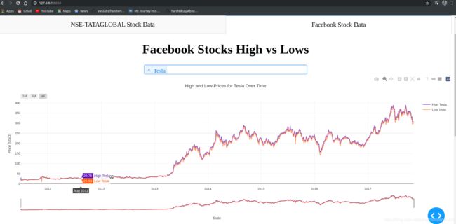
3.分析股票尾市数据

df["Date"]=pd.to_datetime(df.Date,format="%Y-%m-%d")
df.index=df['Date']

plt.figure(figsize=(16,8))
plt.plot(df["Close"],label='Close Price history')

4.构建模型

import math
#Create a new dataframe with only the Close column
data = df.filter(['Close'])
#Convert the dataframe to a numpy array
dataset = data.values

#Get the number of rows to train the model
training_data_len = math.ceil( len(dataset) * .8)
training_data_len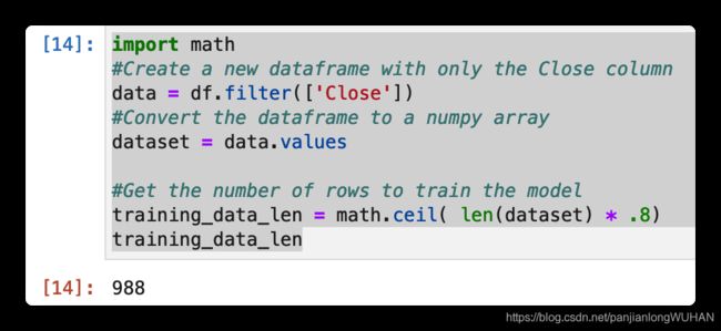

 

#Scale the data
scaler=MinMaxScaler(feature_range=(0,1))
scaled_data=scaler.fit_transform(dataset)

scaled_data

 

#Create the training data set
#Create the scaled training data set
train_data = scaled_data[0:training_data_len , :]
#Split the data into x_train and y_train data sets
x_train = []
y_train = []

for i in range(60,len(train_data)):
    x_train.append(train_data[i-60:i,0])
    y_train.append(train_data[i,0])
    if i<= 60:
        print(x_train)
        print(y_train)
        print()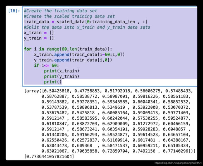

 

#Build the LSTM model
model = Sequential()
model.add(LSTM(50,return_sequences=True,input_shape=(x_train.shape[1],1)))
model.add(LSTM(50,return_sequences=False))
model.add(Dense(25))
model.add(Dense(1))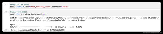

5.测试模型

#Create the testing data set
#Create a new array containing scaled values from index 1543 to 2003
test_data = scaled_data[training_data_len - 60: , :]
#Create the data sets x_test and y_test
x_test = []
y_test = dataset[training_data_len: , :]
for i in range(60, len(test_data)):
    x_test.append(test_data[i-60:i,0])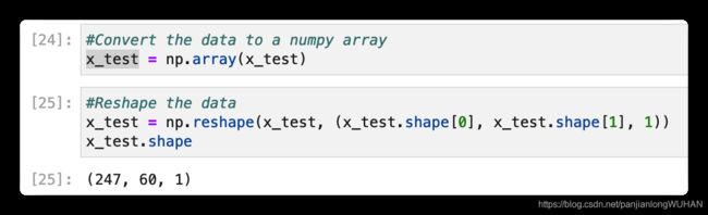

 

#Get the models predicted price values
predictions = model.predict(x_test)
predictions = scaler.inverse_transform(predictions)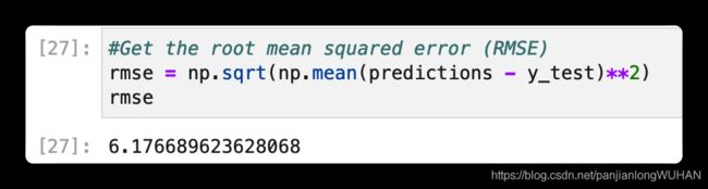

6.展示预测结果

#Plot the data
train = data[:training_data_len]
valid = data[training_data_len:]
valid['Predictions'] = predictions
#Visualize the data
plt.figure(figsize=(16,8))
plt.title('Model')
plt.xlabel('Date', fontsize=18)
plt.ylabel('Close Prise USD ($)', fontsize=18)
plt.plot(train['Close'])
plt.plot(valid[['Close', 'Predictions']])
plt.legend(['Train','Val','Predictions'], loc='lower right')
plt.show()