Tuesday, at the annual meeting of the French Economic Association, I was having lunch Alfred, and while we were chatting about modeling issues (econometric models against machine learning prediction), he asked me what boosting was. Since I could not be very specific, we’ve been looking atwikipedia page.
Boosting is a machine learning ensemble meta-algorithm for reducing bias primarily and also variance in supervised learning, and a family of machine learning algorithms which convert weak learners to strong ones
One should admit that it is not very informative. At least, there is the idea that ‘weak learners’ can be used to get a good predictor. Now, to be honest, I guess I understand the concept. But I still can’t reproduce what I got with standard ‘boosting’ packages.
There are a lot of publications about the concept of ‘boosting’. In 1988, Michael Kearns published Thoughts on Hypothesis Boosting, which is probably the oldest one. About the algorithms, it is possible to find some references. Consider for instance Improving Regressors using Boosting Techniques, by Harris Drucker. Or The Boosting Approach to Machine Learning An Overview by Robert Schapire, among many others. In order to illustrate the use of boosting in the context of regression (and not classification, since I believe it provides a better visualisation) consider the section in Dong-Sheng Cao’s In The boosting: A new idea of building models.
In a very general context, consider a model like

The idea is to write it as

or, as we will seen soon,

(where  ‘s will be some shrinkage parameters). To get all the components of that sum, we will use an iterative procedure. Define the partial sum (that will be our prediction at step
  )
)

Since we consider some regression function here, use the  loss function, to get the function, we solve

(we can imagine that the loss function can be changed, for instance in the context of classification).
The concept is simple, but from a practical perspective, it is actually a difficult problem since optimization is performed here in a very large set (a functional space actually). One of the trick will be to use a base of learners. Weak learners. And to make sure that we don’t use too strong learners, consider also some shrinkage parameters, as discussed previously. The iterative algorithm is
- start with some regression model

- compute the residuals, including some shrinkage parameter,

then the strategy is to model those residuals
- at step
 , consider regression
- update the residuals

and to loop. Then set

So far, I guess I understand the concept. The next step is then to write the code to see how it works, for real. One can easily get the intuition that, indeed, it should work, and we should end up with a decent model. But we have to try it, and play with it to check that it performs better than any other algorithms.
Consider the following dataset,
n=300

set.seed(1)

u=sort(runif(n)*2*pi)

y=sin(u)+rnorm(n)/4

df=data.frame(x=u,y=y)
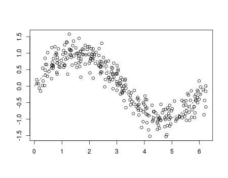
If we visualize it, we get
plot(df)

Consider some linear-by-part regression models. It could make sense here. At each iterations, there are 7 parameters to ‘estimate’, the slopes and the nodes. Here, consider some constant shrinkage parameter (there is no need to start with something to complicated, I guess).
v=.05

library(splines)

fit=lm(y~bs(x,degree=1,df=3),data=df)

yp=predict(fit,newdata=df)

df$yr=df$y - v*yp

YP=v*yp
I store in the original dataset the residuals (that will be updated), and I keep tracks of all the predictions. Consider now the following loop
for(t in 1:100){

  fit=lm(yr~bs(x,degree=1,df=3),data=df)

  yp=predict(fit,newdata=df)

  df$yr=df$yr - v*yp

  YP=cbind(YP,v*yp)

}
This is the implementation of the algorithm described above, right? To visualise it, at some early stage, use
nd=data.frame(x=seq(0,2*pi,by=.01))

viz=function(M){

if(M==1)  y=YP[,1]

if(M>1)   y=apply(YP[,1:M],1,sum)

  plot(df$x,df$y,ylab="",xlab="")

  lines(df$x,y,type="l",col="red",lwd=3)

  fit=lm(y~bs(x,degree=1,df=3),data=df)

  yp=predict(fit,newdata=nd)

  lines(nd$x,yp,type="l",col="blue",lwd=3)

  lines(nd$x,sin(nd$x),lty=2)}
The red line is the initial guess we have, without boosting, using a simple call of the regression function. The blue one is the one obtained using boosting. The dotted line is the truemodel.
viz(50)
Somehow, boosting is working. But even the possibility to get different notes at each step, it looks like we don’t use it. And we cannot perform better than a simple regression function.
What if we use quadratic splines instead of linear splines?
v=.05

fit=lm(y~bs(x,degree=2,df=3),data=df)

yp=predict(fit,newdata=df)

df$yr=df$y - v*yp

YP=v*yp

library(splines)

for(t in 1:100){

  fit=lm(yr~bs(x,degree=2,df=3),data=df)

  yp=predict(fit,newdata=df)

  df$yr=df$yr - v*yp

  YP=cbind(YP,v*yp)

}
Again, boosting is not improving anything here. We’ll discuss later on the impact of the shrinkage parameter, but here, it won’t change much the output (it might be faster of slower to reach the final prediction, but it will always be the same predictive model).
In order to get something different at each step, it tried to add a boostrap procedure. I don’t know if that’s sill ‘boosting’, but why not try it.
v=.1

  idx=sample(1:n,size=n,replace=TRUE)

fit=lm(y~bs(x,degree=1,df=3),data=df[idx,])

yp=predict(fit,newdata=df)

df$yr=df$y - v*yp

YP=v*yp


for(t in 1:100){

  idx=sample(1:n,size=n,replace=TRUE)

fit=lm(yr~bs(x,degree=1,df=3),data=df[idx,])

yp=predict(fit,newdata=df)

df$yr=df$yr - v*yp

YP=cbind(YP,v*yp)

}
At each step, I sample from my dataset, and get a linear-by-parts regression. And again, I use a shrinkage parameter not to learn too fast.
It is slightly different (if you look very carefully). But actually, an algorithm that will be as costly is a ‘bagging’ one, where we boostrap many samples, get different models, and predictions, and then average all the predictions. The (computational) cost is exactly the same here
YP=NULL

library(splines)

for(t in 1:100){

  idx=sample(1:n,size=n,replace=TRUE)

  fit=lm(y~bs(x,degree=1,df=3),data=df[idx,])

  yp=predict(fit,newdata=nd)

  YP=cbind(YP,yp)

}

y=apply(YP[,1:100],1,mean)

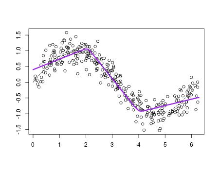
plot(df$x,df$y,ylab="",xlab="")

lines(nd$x,y,type="l",col="purple",lwd=3)

It is very close to what we got with the boosting procedure.
Let us try something else. What if we consider at each step a regression tree, instead of a linear-by-parts regression.
library(rpart)

v=.1

fit=rpart(y~x,data=df)

yp=predict(fit)

df$yr=df$y - v*yp

YP=v*yp

for(t in 1:100){

fit=rpart(yr~x,data=df)

yp=predict(fit,newdata=df)

df$yr=df$yr - v*yp

YP=cbind(YP,v*yp)

}
Again, to visualise the learning process, use
viz=function(M){

y=apply(YP[,1:M],1,sum)

plot(df$x,df$y,ylab="",xlab="")

lines(df$x,y,type="s",col="red",lwd=3)

fit=rpart(y~x,data=df)

yp=predict(fit,newdata=nd)

lines(nd$x,yp,type="s",col="blue",lwd=3)

lines(nd$x,sin(nd$x),lty=2)}
This time, with those trees, it looks like not only we have a good model, but also a different model from the one we can get using a single regression tree.
What if we change the shrinkage parameter?
viz=function(v=0.05){

  fit=rpart(y~x,data=df)

  yp=predict(fit)

  df$yr=df$y - v*yp

  YP=v*yp

  for(t in 1:100){

    fit=rpart(yr~x,data=df)

    yp=predict(fit,newdata=df)

    df$yr=df$yr - v*yp

    YP=cbind(YP,v*yp)

  }

  y=apply(YP,1,sum)

    plot(df$x,df$y,xlab="",ylab="")

    lines(df$x,y,type="s",col="red",lwd=3)

    fit=rpart(y~x,data=df)

    yp=predict(fit,newdata=nd)

    lines(nd$x,yp,type="s",col="blue",lwd=3)

    lines(nd$x,sin(nd$x),lty=2)

}
There is clearly an impact of that parameter. It has to be small to get a good model. This is the idea of using ‘weak learners’ to get a good prediction.
If we add a boostrap sample selection , we get also a good predictive model, here
v=.1

idx=sample(1:n,size=n,replace=TRUE)

fit=rpart(y~x,data=df[idx,])

yp=predict(fit,newdata=df)

df$yr=df$y - v*yp

YP=v*yp

for(t in 1:100){

  idx=sample(1:n,size=n,replace=TRUE)

  fit=rpart(yr~x,data=df[idx,])

  yp=predict(fit,newdata=df)

  df$yr=df$yr - v*yp

  YP=cbind(YP,v*yp)

}
It looks like using a small shrinkage parameter, and some regression tree at each step, we get some ‘weak learners’. It performs well, but so far, I do not see how it could perform better than standard econometric models. But I am still working on it.