100余行代码带你入门强化学习DQN算法
100余行代码带你入门强化学习DQN算法
- 1. 简介
- 2. 关键要点
-
- 2.1 replay buffer存储及采样数据
- 2.2 DQN网络
- 2.3 主函数
- 3. 完整代码
- 4. 关于Nature DQN图像输入的处理手段
1. 简介
DQN算法是经典的强化学习算法, 作为一个入门级的算法,深度强化学习领域的hello world,很有必要自己手动写一个简易实现。
2. 关键要点
DQN算法中,重要的是两个东西,一个是replay buffer,一个是agent。replay buffer涉及到经验的存储与采样。而agent中则涉及到构建神经网络与使用bellman equation更新网络。
2.1 replay buffer存储及采样数据
首先导入必要的库:
import copy
import gym
import torch
import torch.nn as nn
import pandas as pd
import numpy as np
import logging
import sys
import matplotlib.pyplot as plt
replay buffer重要的是两个操作,一个是存储数据,一个是采样数据。在存储数据方面,这里使用pandas.Dataframe来存储,结构清晰,也易于采样。在采样过程中,就采用随机采样的方式。
# ReplayBuffer is used to store transitions which are used to train Q network
class ReplayBuffer:
    def __init__(self, capacity):
        self.capacity = capacity    # record the ReplayBuffer's capacity
        self.valid_count = 0        # record the valid index of transitions
        self.i = 0                  # record the current index which need to store a transition
        # real buffer for storing necessary messages
        self.memory = pd.DataFrame(index=range(capacity),
                                   columns=['state', 'action', 'reward', 'next_state', 'done'])

    def store(self, transition):
        # store the transition
        self.memory.loc[self.i] = transition
        self.i = (self.i+1) % self.capacity     # update the current index which need to store a transition
        self.valid_count = min(self.valid_count+1, self.capacity)       # update the valid index of transitions

    def sample(self, number):
        # choose transitions randomly
        indices = np.random.choice(self.valid_count, size=number)
        return (np.stack(self.memory.loc[indices, var]) for var in self.memory.columns)
2.2 DQN网络
DQN网络重要的是三点,一个是使用epsilon-greedy策略来选择动作(对应get_action方法),一个是从buffer中采样一个batch的transitions来更新Q网络(对应learn方法),一个是硬拷贝更新target Q network(对应update_target_network方法)。因为自己将replay buffer 写在DQN agent中,所以再多一条,是将transtions放入replay buffer中(对应store_transition方法)。
class DQNagent:
    def __init__(self, state_size, action_size, hidden_layer=[16,16]):
        # build the Q network
        layers = []
        for input_size, output_size in zip([state_size,] + hidden_layer, hidden_layer + [action_size,]):
            layers.append(nn.Linear(input_size, output_size))
            layers.append(nn.ReLU())
        layers = layers[:-1]     # delete the last ReLU function
        self.qNet = nn.Sequential(*layers)   # build the Q network
        self.opitimizer = torch.optim.Adam(self.qNet.parameters(), lr=0.001)
        self.loss = nn.MSELoss()

        self.targetQNet = copy.deepcopy(self.qNet)      # build the target Q network
        self.gamma = 0.99                   # discount factor
        self.buffer = ReplayBuffer(10000)
        self.buffer_sample = 1024           # the batch size for training is 1024

        self.lossRecord = []


    def get_action(self, state, action_size, epsilon=0.01):
        # choose the epsilon-greedy action
        state = torch.as_tensor(state, dtype=torch.float)
        with torch.no_grad():
            QValue = self.qNet(state)
        _, act_max = torch.max(QValue, dim=0)
        act = act_max.item() if np.random.rand() > epsilon else np.random.randint(action_size)
        return act

    # store transitions in replay buffer
    def store_transition(self, *transition):
        self.buffer.store(transition)

    # train the Q network
    def learn(self):
        state, action, reward, next_state, done = self.buffer.sample(self.buffer_sample)
        # convert the numpy to torch
        state_tensor = torch.as_tensor(state, dtype=torch.float)
        action_tensor = torch.as_tensor(action, dtype=torch.long)
        reward_tensor = torch.as_tensor(reward, dtype=torch.float)
        next_state_tensor = torch.as_tensor(next_state, dtype=torch.float)
        done_tensor = torch.as_tensor(done, dtype=torch.float)

        predictQ = self.qNet(state_tensor)
        # choose the Q value which is corresponding to the actual action
        q_tensor = predictQ.gather(1, action_tensor.unsqueeze(1)).squeeze(1)

        # calculate the target Q value
        predict_nextQ = self.targetQNet(next_state_tensor)
        predict_next_maxQ, _ = predict_nextQ.max(dim=1)
        targetQ = reward_tensor + (1. - done_tensor) * self.gamma * predict_next_maxQ

        loss = self.loss(targetQ, q_tensor)     # calculate the loss value
        self.lossRecord.append(loss)        # record the loss function
        # three steps for gradient descend
        self.opitimizer.zero_grad()
        loss.backward()
        self.opitimizer.step()

    # update the target network
    def update_target_network(self):
        self.targetQNet = copy.deepcopy(self.qNet)

    # save the Q network model
    def save_model(self, path):
        torch.save(self.qNet.state_dict(), path)

    # load the Q network model
    def load_model(self, path):
        model = torch.load(path)
        self.qNet.load_state_dict(model)

    # draw the training loss curve
    def draw_loss(self):
        plt.figure(1)
        plt.plot(range(len(self.lossRecord)), self.lossRecord)
        plt.xlabel('Training episodes')
        plt.ylabel('loss')
        plt.title('Loss curve during {} training episodes'.format(len(self.lossRecord)))
        plt.savefig('./loss_curve_{}.jpg'.format(len(self.lossRecord)))
2.3 主函数
主函数就是定义环境,然后用agent和环境交互,训练完成后保存模型,之后加载模型并渲染看一下训练效果
if __name__ == '__main__':
    ENV_NAME = "CartPole-v0"
    # show some important messages
    logging.basicConfig(level=logging.DEBUG,
                        format='%(asctime)s [%(levelname)s] %(message)s',
                        stream=sys.stdout, datefmt='%H:%M:%S')
    episodes = 7000
    env = gym.make(ENV_NAME)
    # set random seeds to ensure that the result can be reproduced
    env.seed(0)
    np.random.seed(0)
    torch.manual_seed(0)
    # get the state size and action size of the environment.
    env_state_size, env_action_size = env.observation_space.shape[0], env.action_space.n
    # creat a agent
    agent = DQNagent(env_state_size, env_action_size)
    retList = []
    for i in range(episodes):
        # reset crucial variables
        obs, done, return_aEpisode, steps = env.reset(), False, 0, 0
        while not done:
            action = agent.get_action(obs, env_action_size)     # epsilon-greedy policy.
            obs_new, reward, done, _ = env.step(action)         # interact with the environment
            agent.store_transition(obs, action, reward, obs_new, done)  # collect a transition
            obs = obs_new                                       # update the observation
            return_aEpisode += reward                           # record the return
            steps += 1                                          # record the step
        # if transitions are enough, we begin to update the Q network
        if agent.buffer.valid_count > 0.9 * agent.buffer.capacity:
            agent.learn()
            # update the target Q network every 100 episodes
            if episodes % 100 == 0:
                agent.update_target_network()
        # print key messages
        logging.debug('train episode %d: reward = %.2f, steps = %d',
                      i, return_aEpisode, steps)
        retList.append(return_aEpisode)
    agent.save_model(path='./DQN_{}_model.pth'.format(episodes))        # save trained model
    agent.draw_loss()                                                   # draw the loss curve

    # draw the accumulated reward (i.e. return)
    plt.figure(2)
    plt.plot(range(len(retList)), retList)
    plt.xlabel('episodes')
    plt.ylabel('reward')
    plt.title('interact with the environment in {} episodes'.format(episodes))
    plt.savefig('./reward_curve_{}.jpg'.format(episodes))

    # show the test results
    logging.info('========= test ===========')
    agent.load_model(path='./DQN_{}_model.pth'.format(episodes))
    retList = []
    for i in range(10):
        obs, done, ret = env.reset(), False, 0
        while not done:
            env.render()
            action = agent.get_action(obs, env_action_size)
            obs, reward, done, _ = env.step(action)
            ret += reward
        logging.debug('test episode %d: reward = %.2f',
                          i, ret)
        retList.append(ret)
    env.close()
    logging.info('average episode reward = %.2f ± %.2f',
                np.mean(retList), np.std(retList))
3. 完整代码
import copy
import gym
import torch
import torch.nn as nn
import pandas as pd
import numpy as np
import logging
import sys
import matplotlib.pyplot as plt

# ReplayBuffer is used to store transitions which are used to train Q network
class ReplayBuffer:
    def __init__(self, capacity):
        self.capacity = capacity    # record the ReplayBuffer's capacity
        self.valid_count = 0        # record the valid index of transitions
        self.i = 0                  # record the current index which need to store a transition
        # real buffer for storing necessary messages
        self.memory = pd.DataFrame(index=range(capacity),
                                   columns=['state', 'action', 'reward', 'next_state', 'done'])

    def store(self, transition):
        # store the transition
        self.memory.loc[self.i] = transition
        self.i = (self.i+1) % self.capacity     # update the current index which need to store a transition
        self.valid_count = min(self.valid_count+1, self.capacity)       # update the valid index of transitions

    def sample(self, number):
        # choose transitions randomly
        indices = np.random.choice(self.valid_count, size=number)
        return (np.stack(self.memory.loc[indices, var]) for var in self.memory.columns)


class DQNagent:
    def __init__(self, state_size, action_size, hidden_layer=[16,16]):
        # build the Q network
        layers = []
        for input_size, output_size in zip([state_size,] + hidden_layer, hidden_layer + [action_size,]):
            layers.append(nn.Linear(input_size, output_size))
            layers.append(nn.ReLU())
        layers = layers[:-1]     # delete the last ReLU function
        self.qNet = nn.Sequential(*layers)   # build the Q network
        self.opitimizer = torch.optim.Adam(self.qNet.parameters(), lr=0.001)
        self.loss = nn.MSELoss()

        self.targetQNet = copy.deepcopy(self.qNet)      # build the target Q network
        self.gamma = 0.99                   # discount factor
        self.buffer = ReplayBuffer(10000)
        self.buffer_sample = 1024           # the batch size for training is 1024

        self.lossRecord = []


    def get_action(self, state, action_size, epsilon=0.01):
        # choose the epsilon-greedy action
        state = torch.as_tensor(state, dtype=torch.float)
        with torch.no_grad():
            QValue = self.qNet(state)
        _, act_max = torch.max(QValue, dim=0)
        act = act_max.item() if np.random.rand() > epsilon else np.random.randint(action_size)
        return act

    # store transitions in replay buffer
    def store_transition(self, *transition):
        self.buffer.store(transition)

    # train the Q network
    def learn(self):
        state, action, reward, next_state, done = self.buffer.sample(self.buffer_sample)
        # convert the numpy to torch
        state_tensor = torch.as_tensor(state, dtype=torch.float)
        action_tensor = torch.as_tensor(action, dtype=torch.long)
        reward_tensor = torch.as_tensor(reward, dtype=torch.float)
        next_state_tensor = torch.as_tensor(next_state, dtype=torch.float)
        done_tensor = torch.as_tensor(done, dtype=torch.float)

        predictQ = self.qNet(state_tensor)
        # choose the Q value which is corresponding to the actual action
        q_tensor = predictQ.gather(1, action_tensor.unsqueeze(1)).squeeze(1)

        # calculate the target Q value
        predict_nextQ = self.targetQNet(next_state_tensor)
        predict_next_maxQ, _ = predict_nextQ.max(dim=1)
        targetQ = reward_tensor + (1. - done_tensor) * self.gamma * predict_next_maxQ

        loss = self.loss(targetQ, q_tensor)     # calculate the loss value
        self.lossRecord.append(loss)        # record the loss function
        # three steps for gradient descend
        self.opitimizer.zero_grad()
        loss.backward()
        self.opitimizer.step()

    # update the target network
    def update_target_network(self):
        self.targetQNet = copy.deepcopy(self.qNet)

    # save the Q network model
    def save_model(self, path):
        torch.save(self.qNet.state_dict(), path)

    # load the Q network model
    def load_model(self, path):
        model = torch.load(path)
        self.qNet.load_state_dict(model)

    # draw the training loss curve
    def draw_loss(self):
        plt.figure(1)
        plt.plot(range(len(self.lossRecord)), self.lossRecord)
        plt.xlabel('Training episodes')
        plt.ylabel('loss')
        plt.title('Loss curve during {} training episodes'.format(len(self.lossRecord)))
        plt.savefig('./loss_curve_{}.jpg'.format(len(self.lossRecord)))

if __name__ == '__main__':
    ENV_NAME = "CartPole-v0"
    # show some important messages
    logging.basicConfig(level=logging.DEBUG,
                        format='%(asctime)s [%(levelname)s] %(message)s',
                        stream=sys.stdout, datefmt='%H:%M:%S')
    episodes = 7000
    env = gym.make(ENV_NAME)
    # set random seeds to ensure that the result can be reproduced
    env.seed(0)
    np.random.seed(0)
    torch.manual_seed(0)
    # get the state size and action size of the environment.
    env_state_size, env_action_size = env.observation_space.shape[0], env.action_space.n
    # creat a agent
    agent = DQNagent(env_state_size, env_action_size)
    retList = []
    for i in range(episodes):
        # reset crucial variables
        obs, done, return_aEpisode, steps = env.reset(), False, 0, 0
        while not done:
            action = agent.get_action(obs, env_action_size)     # epsilon-greedy policy.
            obs_new, reward, done, _ = env.step(action)         # interact with the environment
            agent.store_transition(obs, action, reward, obs_new, done)  # collect a transition
            obs = obs_new                                       # update the observation
            return_aEpisode += reward                           # record the return
            steps += 1                                          # record the step
        # if transitions are enough, we begin to update the Q network
        if agent.buffer.valid_count > 0.9 * agent.buffer.capacity:
            agent.learn()
            # update the target Q network every 100 episodes
            if episodes % 100 == 0:
                agent.update_target_network()
        # print key messages
        logging.debug('train episode %d: reward = %.2f, steps = %d',
                      i, return_aEpisode, steps)
        retList.append(return_aEpisode)
    agent.save_model(path='./DQN_{}_model.pth'.format(episodes))        # save trained model
    agent.draw_loss()                                                   # draw the loss curve

    # draw the accumulated reward (i.e. return)
    plt.figure(2)
    plt.plot(range(len(retList)), retList)
    plt.xlabel('episodes')
    plt.ylabel('reward')
    plt.title('interact with the environment in {} episodes'.format(episodes))
    plt.savefig('./reward_curve_{}.jpg'.format(episodes))

    # show the test results
    logging.info('========= test ===========')
    agent.load_model(path='./DQN_{}_model.pth'.format(episodes))
    retList = []
    for i in range(10):
        obs, done, ret = env.reset(), False, 0
        while not done:
            env.render()
            action = agent.get_action(obs, env_action_size)
            obs, reward, done, _ = env.step(action)
            ret += reward
        logging.debug('test episode %d: reward = %.2f',
                          i, ret)
        retList.append(ret)
    env.close()
    logging.info('average episode reward = %.2f ± %.2f',
                np.mean(retList), np.std(retList))
4. 关于Nature DQN图像输入的处理手段
在2015年发表在nature上的DQN算法是使用图像作为状态输入,使用了卷积神经网络。而这里我写的DQN算法是通过gym的接口拿到的状态,并不涉及到图像理解,这种也称为侵入式算法(就是从仿真器底层拿到了状态数据)。
对于纯图像理解的非侵入式算法,我们来看看DQN是如何做的,这里只重点讲输入图像的预处理(我看了nature的论文,感觉讲得不是很清楚,所以自己找了些资料,重新描述一遍),网络结构可以直接参考nature论文(其实就是用于分类的卷积神经网络结构)
首先为了减少计算量,将原彩色RGB图片变为亮度图,且将 210 × 160 210 \times160 210×160尺寸的图片压缩为 84 × 84 84 \times 84 84×84。此外,还采用了跳帧技术,每隔4帧采2张图片。
然后对于Atari游戏中会出现“闪动”的情况(即有些物体只在偶数帧出现,有些物体只在奇数帧出现,但是他们又实际存在),Nature DQN的做法是两张连续帧的图片逐像素比较取较大值,从而两张连续帧就变为了一帧。不妨记为 x i x_i xi。
最后再考虑到agent计算一个动作的时间大于环境变化一次的时间,且为了和人类公平比较(毕竟人类的反应速度有上限),Nature DQN隔固定帧数才采取一个动作,在这些帧期间,动作恒定不变。
那么Nature DQN的状态输入 s t = ( x t − 3 , x t − 2 , x t − 1 , x t ) s_t = (x_{t-3}, x_{t-2}, x_{t-1}, x_{t}) st=(xt−3,xt−2,xt−1,xt),即状态输入的维数为 4 × 84 × 84 4 \times 84 \times 84 4×84×84,然后把它送入到卷积神经网络中。
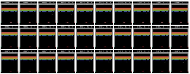
前面的表述可能有些抽象,看下面的图更加直观。下图中的打叉部分为跳过的帧,而黄色框框柱的为两帧合为一帧的 x i x_i xi部分,那么 x 1 , x 2 , x 3 , x 4 x_1, x_2, x_3, x_4 x1,x2,x3,x4堆叠到一起就组成了状态 s 4 s_4 s4,然后通过DQN网络计算得到动作 a 4 a_4 a4,接下来的四帧采用动作 a 4 a_4 a4进行环境交互,然后我们能得到 x 5 x_5 x5,而 x 2 , x 3 , x 4 , x 5 x_2, x_3, x_4, x_5 x2,x3,x4,x5堆叠到一起就组成了状态 s 5 s_5 s5,如此往复下去。

图片来源:
https://danieltakeshi.github.io/2016/11/25/frame-skipping-and-preprocessing-for-deep-q-networks-on-atari-2600-games/