在数学空间中,物理分辨率可能失去了意义(behind the paper)
写在前面:2020-01到2021-07于我来说,是非常艰难的两年,所以这段时间一直也没有在CSDN持续整理/转载一些CV知识了。而这期间经历了4~5轮审稿,从nature辗转nature biotechnology,终于把第一篇工作发表了出来,感兴趣的可以看这个链接(Sparse deconvolution improves the resolution of live-cell super-resolution fluorescence microscopy | Nature Biotechnology)
这篇文章,其实是我发表在 Nature Research Bioengineering Community的一篇英文博文,分享一些对文章中方法的一些基本的理解和思考,我就直接转载到了CSDN平台,just some personal thoughts to share, hope this helps.
---------------------------------------------------------------------------------------------------------------------------------
Start point (Physics->Chemistry->Mathematics?)
When I started my Ph.D. in 2017, I began to dig into the field of super-resolution microscopy which was already Nobel prize rewarded and well-established at that time. The start point of super-resolution microscopy, I thought, is the higher-NA/shorter-wavelength configurations and the confocal concept, which are pure physical methods to improve the resolution. Restricted by the real physical conditions, the corresponding resolution improvements were very limited. As time goes on, more and more fluorescence markers are being developed, the microscopists are beginning to be dissatisfied with such pure physical methods, and move on to the indirect chemical strategies, i.e., the fluorescence superresolution microscopies (SMLM/STED). However, all these methods need to sacrifice something in exchange for the resolution improvement.
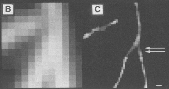
On the other hand, I found the mathematical algorithms, in particular the deconvolution method is conceptually a quite straightforward and generalized approach to improve the resolution:
(Fig.3B, 3C from Superresolution Three-Dimensional Images of Fluorescence in Cells with Minimal Light Exposure | Science)
Actually, broadly speaking, most computational super-resolution methods contain the core concept of deconvolution, which is to decode real signals from measured signals. Unfortunately, although deconvolution has been routinely used for image enhancement, and even commonly involved as an auxiliary function in most commercial microscope systems, so far the idea that deconvolution can directly achieve super-resolution does not seem to be widely accepted by the community.
If considering that most conventional deconvolution methods have very limited performance and strict requirements on signal-to-noise ratio and sampling rate, we found that this prejudice will be quite predictable and acceptable. If there are deconvolution methods consistently unsensitive to noise and highly efficient at decoding high-frequency information, we thought this may broke the bias of community.
This post hopes to share some fundamental discussions on deconvolution methodsand some bottom-up insights of how we designed the sparse deconvolution. For me, the development roadmap of optical super-resolution microscopy can be written as:
Physics (~1970) -> Chemistry(~2010) -> Mathematics (~2020)
(Ill-posed?) Inverse problem
Interestingly, without noise and with infinite sampling rate, even if the image is blurred by a PSF, we can still recover the real signal precisely. To clarify this point, I will next provide a little background of the inverse problem and deconvolution. For me, the deconvolution is actually a classical machine learning method, rather than an optical method, that estimate the hidden parameter (real signal) from the measured parameter (camera image).
Ax = y. It is an inverse problem if without noise.
Sampling{Ax + n} = y. It is an ill-posed inverse problem if with noise and sampling.
What we’re doing is trying to estimate the maximum possible x from the observed data y. If the A is a gaussian-function/point-source, and under noise-free condition, the x and y can be one–to–one correspondence.
In the field of machine learning or convex optimization, before establishing a model, we always start by asking ourselves, is this problem convex, or is there existing a global optimum. If there is no noise, then the x and y can be one–to–one correspondence. No matter what method we use, we just need to find x that Ax is absolutely equal to y.
There are many solutions, including the Bayesian-based Richardson-Lucy (RL) deconvolution, which will be discussed below. If the computing power is sufficient, even particle swarm (PSO) or genetic algorithm (GA) are effective choices. We can define the x as the parameters to be optimized by GA/PSO, and the optimization will stop when find x for Ax – y = 0.
Noise-free simulation
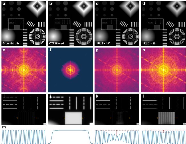
In Supplementary Fig. 1, without noise and down-sampling, even using the band-limited PSF, RL can recover the missing information.
"In this sense, physical resolution might be meaningless if in the mathmetical space."
(Supplementary Fig. 1 from our work Sparse deconvolution improves the resolution of live-cell super-resolution fluorescence microscopy | Nature Biotechnology)
Low-pass filtered image recovered by RL deconvolution under noise-free condition. (a) The ground-truth contains synthetic various-shaped structures with a pixel size of 20 nm. (b) The low-pass filtered (equal to 90 nm resolution) image of (a). (c) RL deconvolution result of (b) with 2×10⁴ iterations. (d) RL deconvolution with 2×10⁷iterations. (e-h) Fourier transforms of (a-d). (i-l) Magnified views of white boxes from (a-d). (m) The corresponding profiles are taken from the regions between the yellow arrowheads in (i-l).
Prior knowledge
From a Bayesian perspective, introducing additional reasonable prior knowledge will make the estimation for small datasets (low photon number, small OTF support) more effective.
For example: Considering the image contained background noise, if corresponding to maximum likelihood estimation (MLE), RL only considers Poisson noise, while Poisson noise does not contain background. So, the RL model seems to be deviating from the range of application (the image with background). It would be a good correction/prior-knowledge to add b to the model based on this definition.
Of course, it is extremely complex in real world, including Gaussian-Poisson noise, background noise, defocus signal, cytosol signal, and limited sampling (pixel-size). The regularization function is necessary for obtaining a unique solution in under-constrained systems.
argmin{L (x, y) + λ × R(x)},
where y is the raw image, x is the reconstructed image, L(·,·) is the data fitting loss between the measured data and the forward model prediction, R(·) is a regularization function on the image, and λ is the hyper-parameter balancing the data fitting loss and the regularization term.
It is always a good way to add the corresponding prior knowledge to power the estimation. This word might be not restricting to deconvolution but all algorithms.
Taken an example of single molecular localization microscopy (SMLM), which can also be treated as a deconvolution method, it utilizes the strongest prior knowledge on the real fluorescent signal x, i.e., the isolate puncta, to achieve super-resolution in 10~20 times. However, the usage of such prior knowledge needs the specific designed experiment, and can not be applied to the conventional microscopes.
Sparse deconvolution
Before moving on to our most important prior knowledge, I intend to say that in the field of machine learning, loss functions are the soul of the methods. This is also the basis for judging whether the prior knowledge is effective. Whether the desired effect [increased resolution in deconvolution] can reduce the loss function with prior knowledge added. If it does, it’s effective for this objective.
What we intend to do is to find the relatively weak but general (for fluorescence imaging) prior-knowledge in the manuscript:
- PSF is an important prior knowledge, the soul of deconvolution.
- Sparsity, we used the L1 norm as a start point (the sum of the absolute values of all the elements). From the forward model of fluorescence imaging, a smaller PSF convolution corresponds to a smaller L1 norm loss function. At least if the forward model of fluorescence imaging is satisfied, then this prior is reasonable.
- Continuity, we used the Hessian matrix norm (the sum of the absolute values of the second order derivative). The notation is [1,-2, 1] as in x direction. The PSF of images must occupy more than 3 × 3 pixels in space which constitutes the basis for the continuity. At least if the Nyquist sampling criteria of images is satisfied, then this prior is reasonable.
- Low frequency background, corresponding to cytosol signal and constant background. This is an optional priori knowledge.
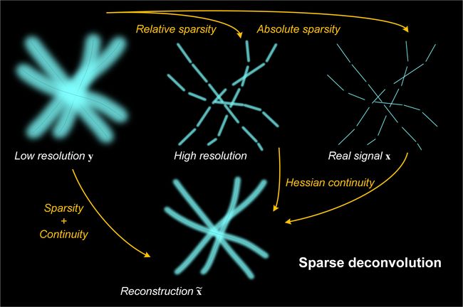
Thus, sparsity recovers the high frequency information (towards to the real signal), and in the meantime the image is also constrained by the Hessian matrix continuity. As these priors on two different levels recovering the signal cooperatively, the proposed sparse deconvolution is more robust and effective. Here we provide an abstract working process of our sparse deconvolution:
Visual examples
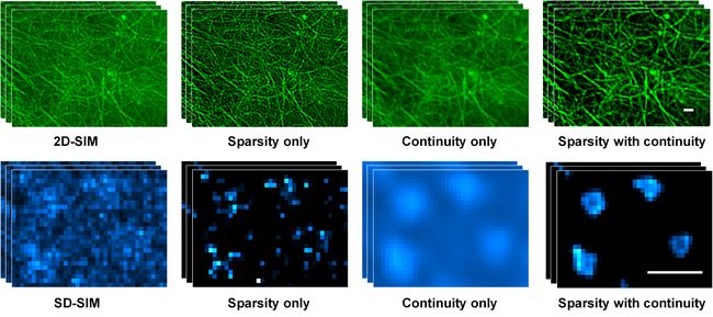
Here we provide two examples to illustrate the different effects from different prior knowledge:
(Supplementary Fig. 3d from our work Sparse deconvolution improves the resolution of live-cell super-resolution fluorescence microscopy | Nature Biotechnology)
The concept of sparse deconvolution. (d) Reconstructions with only sparsity, only continuity, or both the sparsity and continuity priors. Actin filaments labeled with LifeAct-EGFP in a live COS-7 cell in Fig. 4a under 2D-SIM (left, top panel) and CCPs labeled by Clathrin-EGFP in Fig. 5a under SD-SIM (left, bottom panel), followed by sparsity-constraint deconvolution (middle left), continuity-constraint deconvolution (middle right), or both sparsity and continuity-constraint deconvolution (right). Scale bars: 500 nm.
We have tested our sparse deconvolution on various miscoscopes and diverse samples:
(Supplementary Fig. 4 from our work Sparse deconvolution improves the resolution of live-cell super-resolution fluorescence microscopy | Nature Biotechnology)
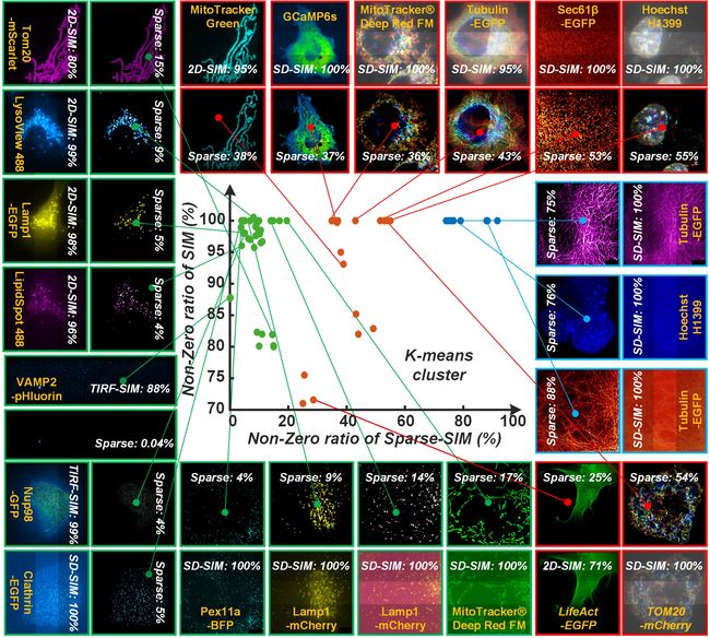
Different decreases in non-zero ratios of images after the sparse deconvolution. We collected the number of non-zero values of images of this paper before and after our sparse deconvolution (details also in Supplementary Table 4). To demonstrate these numbers more clearly, they are normalized by the total pixel number of images. The resulting ratios could be clustered by the K-means method30 into three categories in different colors (green, red, and blue). Each scatter denotes a non-zero ratio of one frame before (x-axis) and after (y-axis) the sparse deconvolution.
Outlook
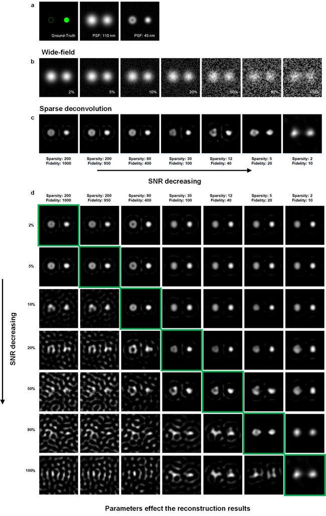
Admittedly, the reasonable usage of prior knowledge is a prerequisite for the method to really apply to the biological applications. Unreasonable parameters do lead to less-than-ideal results.
- For example, infinitely increasing the parameter of sparsity will turn the whole picture into zero. The loss function will be equal to the
L1 normonly. - See also the following specific simulation example:
Simulations under different SNR, and the corresponding reconstruction results. (a) We created synthetic ring-shaped and punctated structures with an 80 nm diameter as ground-truth (left). It was convolved with PSF with FWHM of either 110 nm (middle) or 45 nm (right). (b) These images were subsequently subsampled 16 times (pixel sizes of 16 nm), and corrupted with Poisson noise and 2%, 5%, 10%, 20%, 50%, 80%, and 100% Gaussian noise. (c) The images with different Gaussian noise amplitudes are processed with different weights of priors. (d) The 7 × 7 table of the reconstruction results. The column, and row represent the noise amplitude and weights of priors for reconstruction, respectively.
Although it still has its disadvantages (a little bit more tunable parameters), we believe that sparse deconvolution is currently the best and the most effective solution/method. Under a broader perspective, this is probably the TOP method of generative models in the field of unsupervised learning (including deep or non-deep methods) for fluorescence image restoration.
All technologies have its boundaries, and using proof by contradiction to evaluate them might be not appropriate. The success is success, the unsuccessful example will only illustrate the boundary of the technology. Just as all microscopes are suitable for imaging only a certain range of samples.
The unrestricted using and testing can lead to the strange results. But we are eager for the community to test it extensively, and exploring the boundaries of this method, which will also give us or other developers the opportunity to push the algorithm limit further.
Open source
HERE you can find the source codes of sparse deconvolution to reproduce our results.
HERE you can access more results and comparisons on my website.
