笔记:Deep learning for time series classification: a review
1 Introduction
- This paper targets the following open questions:
- What is the current state-of-the-art DNN for TSC?
- Is there a current DNN approach that reaches state-of-the-art performance for TSC and is less complex than HIVE-COTE?
- What type of DNN architectures works best for the TSC task?
- How does the random initialization affect the performance of deep learning classifiers?
- Could the black-box effect of DNNs be avoided to provide interpretability?
- The main contributions of this paper can be summarized as follows:
- We explain with practical examples, how deep learning can be adapted to one dimensional time series data.
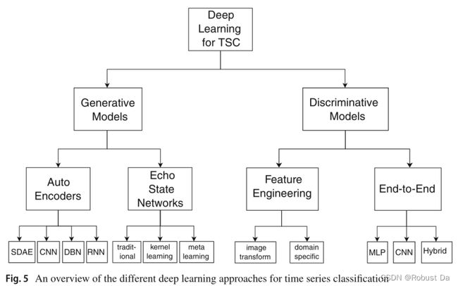
- We propose a unified taxonomy that regroups the recent applications of DNNs for TSC in various domains under two main categories: generative and discriminative models.
- We detail the architecture of nine end-to-end deep learning models designed specifically for TSC.
- We evaluate these models on the univariate UCR/UEA archive benchmark and 12 MTS classification datasets.
- We provide the community with an open source deep learning framework for TSC in which we have implemented all nine approaches.
- We investigate the use of Class Activation Map (CAM) in order to reduce DNNs’ black-box effect and explain the different decisions taken by various models.
2 Background
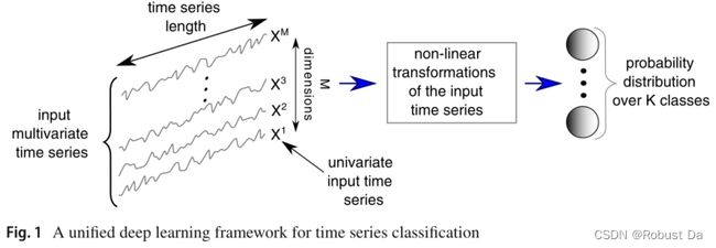
- A general deep learning framework for TSC is depicted in Fig. 1. These networks are designed to learn hierarchical representations of the data.
- In this review we focus on three main DNN architectures used for the TSC task: Multi Layer Perceptron (MLP), Convolutional Neural Network (CNN) and Echo State Network (ESN).
2.2 Deep learning for time series classification
2.2.1 Multi layer perceptrons
- An MLP constitutes the simplest and most traditional architecture for deep learning models.
- One impediment(阻碍) from adopting MLPs for time series data is that they do not exhibit any spatial invariance. In other words, each time stamp has its own weight and the temporal information is lost: meaning time series elements are treated independently from each other.
2.2.2 Convolutional neural networks
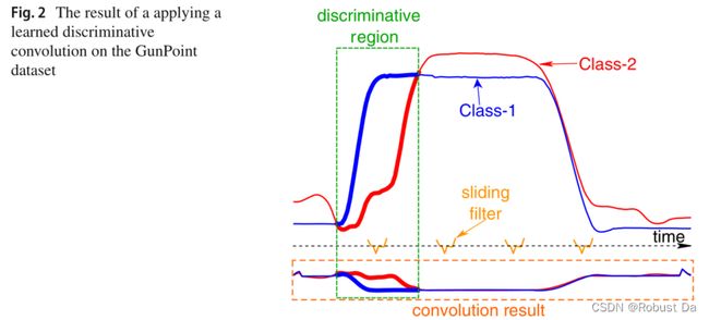
- A convolution can be seen as applying and sliding a filter over the time series. Unlike images, the filters exhibit only one dimension (time) instead of two dimensions (width and height). The filter can also be seen as a generic non-linear transformation of a time series.
- Unlike MLPs, the same convolution (the same filter values w and b) will be used to find the result for all time stamps t ∈ [1, T]. This is a very powerful property (called weight sharing) of the CNNs which enables them to learn filters that are invariant across the time dimension.
2.2.3 Echo state networks
- Another popular type of architectures for deep learning models is the Recurrent Neural Network (RNN).
- Apart from time series forecasting, we found that these neural networks were rarely applied for time series classification which is mainly due to three factors: (1) the type of this architecture is designed mainly to predict an output for each element (time stamp) in the time series (Längkvist et al. 2014); (2) RNNs typically suffer from the vanishing gradient problem due to training on long time series (Pascanu et al. 2012); (3) RNNs are considered hard to train and parallelize which led the researchers to avoid using them for computational reasons (Pascanu et al. 2013).
- Given the aforementioned limitations, a relatively recent type of recurrent architecture was proposed for time series: Echo State Networks (ESNs) (Gallicchio and Micheli 2017).
- To better understand the mechanism of these networks, consider an ESN with input dimensionality M, neurons in the reservoir Nr and an output dimensionality K equal to the number of classes in the dataset. Let X(t) ∈ RM, I(t) ∈ RNr and Y(t) ∈ RK denote the vectors of the input M-dimensional MTS, the internal (or hidden) state and the output unit activity for time t respectively. Further let Win ∈ RNr×M and W ∈ RNr×Nr and Wout ∈ RC×Nr denote respectively the weight matrices for the input time series, the internal connections and the output connections as seen in Fig. 4. The internal unit activity I(t) at time t is updated using the internal state at time step t−1 and the input time series element at time t. Formally the hidden state can be computed using the following recurrence:

with f denoting an activation function of the neurons, a common choice is tanh(·) applied element-wise (Tanisaro and Heidemann 2016). The output can be computed according to the following equation:

thus classifying each time series element X(t). Note that ESNs depend highly on the initial values of the reservoir that should satisfy a pre-determined hyperparameter: the spectral radius. Fig. 4 shows an example of an ESN with a univariate input time series to be classified into K classes.
2.3 Generative or discriminative approaches
2.3.1 Generative models
- Generative models usually exhibit an unsupervised training step that precedes(在……之前) the learning phase of the classifier (Längkvist et al. 2014).This type of network has been referred to as Model-based classifiers in the TSC community (Bagnall et al. 2017).
- For all generative approaches, the goal is to find a good representation of time series prior to training a classifier (Längkvist et al. 2014).
2.3.2 Discriminative models
- A discriminative deep learning model is a classifier (or regressor) that directly learns the mapping between the raw input of a time series (or its hand engineered features) and outputs a probability distribution over the class variables in a dataset.
- This type of model could be further sub-divided into two groups: (1) deep learning models with hand engineered features and (2) end-to-end deep learning models.
- The most frequently encountered and computer vision inspired feature extraction method for hand engineering approaches is the transformation of time series into images using specific imaging methods such as Gramian fields (Wang and Oates 2015b, a), recurrence plots (Hatami et al. 2017; Tripathy and Acharya 2018) and Markov transition fields (Wang and Oates 2015c).
- Unlike image transformation, other feature extraction methods are not domain agnostic. These features are first hand-engineered using some domain knowledge, then fed to a deep learning discriminative classifier.
- In contrast to feature engineering, end-to-end deep learning aims to incorporate the feature learning process while fine-tuning the discriminative classifier (Nweke et al. 2018). Since this type of deep learning approach is domain agnostic and does not include any domain specific pre-processing steps, we decided to further separate these end-to-end approaches using their neural network architectures.
- This type of deep learning approach is domain agnostic and does not include any domain specific pre-processing steps.
- During our study, we found that CNN is the most widely applied architecture for the TSC problem, which is probably due to their robustness and the relatively small amount of training time compared to complex architectures such as RNNs or MLPs.
3 Approaches
- The main goal of deep learning approaches is to remove the bias due to manually designed features (Ordó¨nez and Roggen 2016), thus enabling the network to learn the most discriminant useful features for the classification task.
3.2.1 Multi layer perceptron
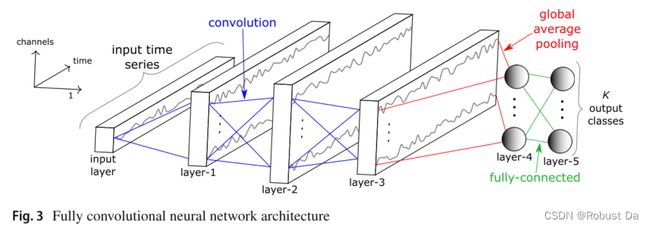
3.2.2 Fully convolutional neural network
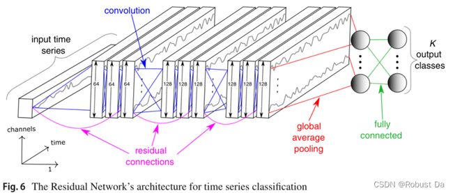
3.2.3 Residual network
3.2.4 Encoder
- Originally proposed by Serrà et al. (2018), Encoder is a hybrid deep CNN whose architecture is inspired by FCN (Wang et al. 2017b) with a main difference where the GAP layer is replaced with an attention layer.
3.2.5 Multi-scale convolutional neural network
3.2.6 Time Le-Net
3.2.7 Multi channel deep convolutional neural network
3.2.8 Time convolutional neural network
3.2.9 Time warping invariant echo state network
4 Experimental setup
4.1 Datasets
4.1.1 Univariate archive
- UCR/UEA archive (Chen et al. 2015b; Bagnall et al. 2017) which contains 85 univariate time series datasets.
- The datasets possess different varying characteristics such as the length of the series which has a minimum value of 24 for the ItalyPowerDemand dataset and a maximum equal to 2709 for the HandOutLines dataset.
4.1.2 Multivariate archive
- Baydogan’s archive (Baydogan 2015) that contains 13 MTS classification datasets.
5 Results
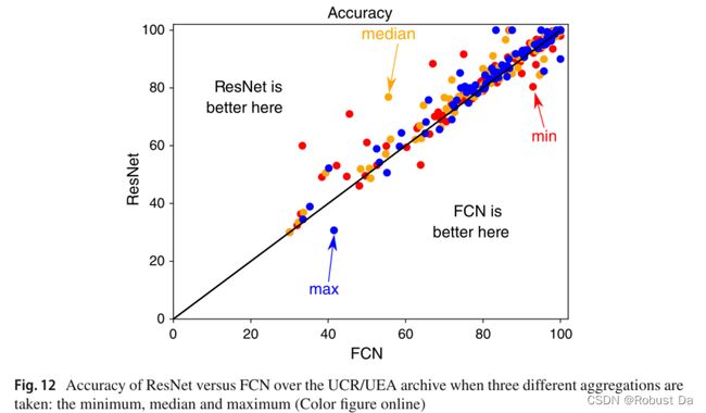
ResNet is relatively better.
6 Visualization
6.1 Class activation map
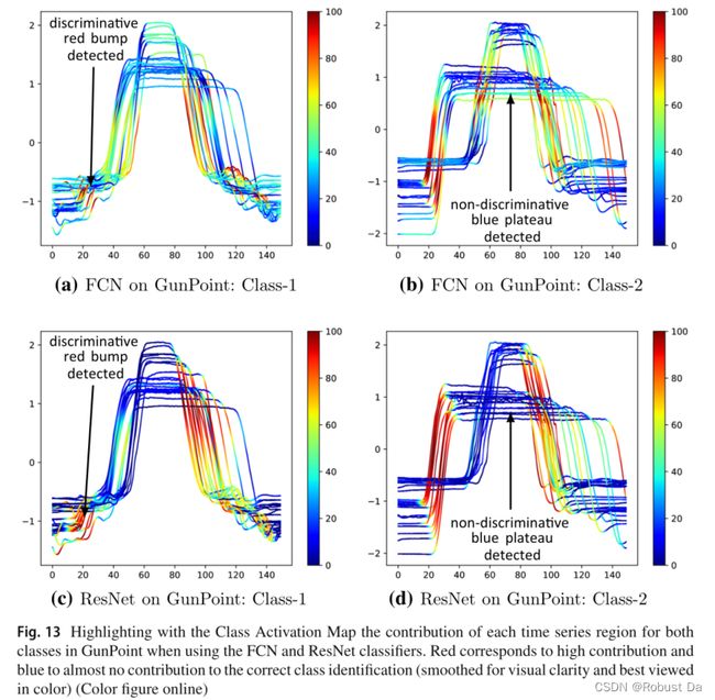
- We investigate the use of Class Activation Map (CAM) which was first introduced by Zhou et al. (2016) to highlight the parts of an image that contributed the most for a given class identification. Wang et al. (2017b) later introduced a one-dimensional CAM with an application to TSC. This method explains the classification of a certain deep learning model by highlighting the subsequences that contributed the most to a certain classification.
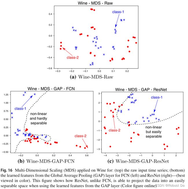
6.2 Multi-dimensional scaling
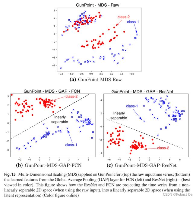
- We propose the use of Multi-Dimensional Scaling (MDS) (Kruskal and Wish 1978) with the objective to gain some insights on the spatial distribution of the input time series belonging to different classes in the dataset.
