大模型系列:OpenAI使用技巧_自定义文本向量化embeding
文章目录
-
- 0. Imports
- 1. 输入
- 2. 加载和处理输入数据
- 3. 将数据分成训练和测试集
- 4. 生成合成的负样本
- 5. 计算嵌入和余弦相似度
- 6. 绘制余弦相似度的分布图
- 7. 使用提供的训练数据优化矩阵。
- 8. 绘制训练期间找到的最佳矩阵的前后对比图,展示结果
本笔记本演示了一种将OpenAI嵌入定制为特定任务的方法。
输入是以[text_1,text_2,label]形式的训练数据,其中label为+1表示这些句子对相似,label为-1表示这些句子对不相似。
输出是一个矩阵,您可以用它来乘以您的嵌入。这个乘法的结果是一个“自定义嵌入”,它将更好地强调与您的用例相关的文本方面。在二元分类用例中,我们看到错误率下降了多达50%。
在下面的示例中,我使用了从SNLI语料库中选择的1,000个句子对。每对句子在逻辑上是蕴含的(即一个句子暗示着另一个句子)。这些句子对是我们的正例(label = 1)。我们通过组合来自不同句子对的句子来生成合成的负例,这些句子被认为不是逻辑上蕴含的(label = -1)。
对于聚类用例,您可以通过从相同聚类中的文本创建句子对来生成正例,并通过从不同聚类中的句子创建句子对来生成负例。
对于其他数据集,我们发现即使只有大约100个训练示例,也能看到相当不错的改进。当然,使用更多示例性能会更好。
0. Imports
# 导入所需的库
from typing import List, Tuple  # 用于类型提示

import numpy as np  # 用于操作数组
import pandas as pd  # 用于操作数据框
import pickle  # 用于保存嵌入缓存
import plotly.express as px  # 用于绘图
import random  # 用于生成运行ID
from sklearn.model_selection import train_test_split  # 用于拆分训练和测试数据
import torch  # 用于矩阵优化

from utils.embeddings_utils import get_embedding, cosine_similarity  # 用于嵌入
1. 输入
大部分的输入都在这里。需要改变的关键点是从哪里加载数据集,将嵌入缓存保存到哪里,以及你想要使用哪个嵌入引擎。
根据你的数据格式,你可能需要重写process_input_data函数。
# 输入参数
embedding_cache_path = "data/snli_embedding_cache.pkl"  # 嵌入将被保存/加载到这里
default_embedding_engine = "babbage-similarity"  # 推荐使用text-embedding-ada-002
num_pairs_to_embed = 1000  # 1000是任意的
local_dataset_path = "data/snli_1.0_train_2k.csv"  # 从以下网址下载:https://nlp.stanford.edu/projects/snli/

def process_input_data(df: pd.DataFrame) -> pd.DataFrame:
    # 你可以自定义这个函数来预处理你自己的数据集
    # 输出应该是一个包含3列的DataFrame:text_1, text_2, label (相似为1,不相似为-1)
    df["label"] = df["gold_label"]  # 将gold_label列的值赋给label列
    df = df[df["label"].isin(["entailment"])]  # 保留label列值为"entailment"的行
    df["label"] = df["label"].apply(lambda x: {"entailment": 1, "contradiction": -1}[x])  # 将label列的值映射为1或-1
    df = df.rename(columns={"sentence1": "text_1", "sentence2": "text_2"})  # 将列名sentence1改为text_1,将列名sentence2改为text_2
    df = df[["text_1", "text_2", "label"]]  # 保留text_1、text_2和label这三列
    df = df.head(num_pairs_to_embed)  # 保留前num_pairs_to_embed行
    return df  # 返回处理后的DataFrame
2. 加载和处理输入数据
# 加载数据
df = pd.read_csv(local_dataset_path)

# 处理输入数据
df = process_input_data(df)  # 这个函数演示了只包含正例的训练数据

# 查看数据
df.head()
/var/folders/r4/x3kdvs816995fnnph2gdpwp40000gn/T/ipykernel_17509/1977422881.py:13: SettingWithCopyWarning:
A value is trying to be set on a copy of a slice from a DataFrame.
Try using .loc[row_indexer,col_indexer] = value instead

See the caveats in the documentation: https://pandas.pydata.org/pandas-docs/stable/user_guide/indexing.html#returning-a-view-versus-a-copy
  df["label"] = df["label"].apply(lambda x: {"entailment": 1, "contradiction": -1}[x])
| text_1 | text_2 | label | |
|---|---|---|---|
| 2 | A person on a horse jumps over a broken down a... | A person is outdoors, on a horse. | 1 |
| 4 | Children smiling and waving at camera | There are children present | 1 |
| 7 | A boy is jumping on skateboard in the middle o... | The boy does a skateboarding trick. | 1 |
| 14 | Two blond women are hugging one another. | There are women showing affection. | 1 |
| 17 | A few people in a restaurant setting, one of t... | The diners are at a restaurant. | 1 |
3. 将数据分成训练和测试集
请注意,在生成合成的负面或正面之前,将数据分成训练和测试集非常重要。您不希望训练数据中的任何文本字符串出现在测试数据中。如果有污染,测试指标看起来会比实际生产中要好。
# 将数据分割为训练集和测试集
test_fraction = 0.5  # 测试集所占比例为0.5,这个值是相对随意的
random_seed = 123  # 随机种子是随意的,但有助于结果的可重复性
train_df, test_df = train_test_split(
    df, test_size=test_fraction, stratify=df["label"], random_state=random_seed
)
# 将训练集的"dataset"列设置为"train"
train_df.loc[:, "dataset"] = "train"
# 将测试集的"dataset"列设置为"test"
test_df.loc[:, "dataset"] = "test"
4. 生成合成的负样本
这是代码的另一部分,您需要根据您的用例进行修改。
如果您的数据中有正样本和负样本,您可以跳过本节。
如果您的数据只有正样本,您可以大部分保持原样,只生成负样本。
如果您的数据是多类别数据,您将希望生成正样本和负样本。正样本可以是共享标签的文本对,而负样本可以是不共享标签的文本对。
最终输出应该是一个带有文本对的数据框,每个对都有标签-1或1。
# 生成负样本

def dataframe_of_negatives(dataframe_of_positives: pd.DataFrame) -> pd.DataFrame:
    """通过组合正样本的元素,返回负样本的数据框。"""

    # 获取所有文本的集合
    texts = set(dataframe_of_positives["text_1"].values) | set(
        dataframe_of_positives["text_2"].values
    )

    # 生成所有可能的文本对
    all_pairs = {(t1, t2) for t1 in texts for t2 in texts if t1 < t2}

    # 获取正样本的文本对
    positive_pairs = set(
        tuple(text_pair)
        for text_pair in dataframe_of_positives[["text_1", "text_2"]].values
    )

    # 生成负样本的文本对
    negative_pairs = all_pairs - positive_pairs

    # 将负样本的文本对转换为数据框
    df_of_negatives = pd.DataFrame(list(negative_pairs), columns=["text_1", "text_2"])

    # 添加标签列,标记为-1表示负样本
    df_of_negatives["label"] = -1

    return df_of_negatives
# 设置每个正样本对应的负样本数量
negatives_per_positive = (
    1  # 可以使用更高的值,但是会导致数据量增加,训练速度变慢
)

# 为训练数据集生成负样本
train_df_negatives = dataframe_of_negatives(train_df)
train_df_negatives["dataset"] = "train"  # 为负样本添加一个"dataset"列,值为"train"

# 为测试数据集生成负样本
test_df_negatives = dataframe_of_negatives(test_df)
test_df_negatives["dataset"] = "test"  # 为负样本添加一个"dataset"列,值为"test"

# 从负样本中随机抽样,并与正样本合并
train_df = pd.concat(
    [
        train_df,
        train_df_negatives.sample(
            n=len(train_df) * negatives_per_positive, random_state=random_seed
        ),
    ]
)

# 从负样本中随机抽样,并与正样本合并
test_df = pd.concat(
    [
        test_df,
        test_df_negatives.sample(
            n=len(test_df) * negatives_per_positive, random_state=random_seed
        ),
    ]
)

# 将训练数据集和测试数据集合并为一个数据集
df = pd.concat([train_df, test_df])
5. 计算嵌入和余弦相似度
在这里,我创建了一个缓存来保存嵌入。这样做很方便,因为如果您想再次运行代码,就不必再次付费。
# 建立一个嵌入缓存以避免重新计算
# 缓存是一个元组(text, engine) -> embedding的字典
try:
    with open(embedding_cache_path, "rb") as f:
        embedding_cache = pickle.load(f) # 从文件中读取缓存
except FileNotFoundError:
    precomputed_embedding_cache_path = "https://cdn.openai.com/API/examples/data/snli_embedding_cache.pkl"
    embedding_cache = pd.read_pickle(precomputed_embedding_cache_path) # 如果文件不存在,则从预计算的缓存中读取

# 这个函数将从缓存中获取嵌入并保存它们
def get_embedding_with_cache(
    text: str,
    engine: str = default_embedding_engine,
    embedding_cache: dict = embedding_cache,
    embedding_cache_path: str = embedding_cache_path,
) -> list:
    if (text, engine) not in embedding_cache.keys(): # 如果缓存中没有,则调用API获取嵌入
        embedding_cache[(text, engine)] = get_embedding(text, engine)
        # 每次更新后将嵌入缓存保存到磁盘
        with open(embedding_cache_path, "wb") as embedding_cache_file:
            pickle.dump(embedding_cache, embedding_cache_file)
    return embedding_cache[(text, engine)]

# 创建嵌入列
for column in ["text_1", "text_2"]:
    df[f"{column}_embedding"] = df[column].apply(get_embedding_with_cache)

# 创建嵌入之间余弦相似度的列
df["cosine_similarity"] = df.apply(
    lambda row: cosine_similarity(row["text_1_embedding"], row["text_2_embedding"]),
    axis=1,
)
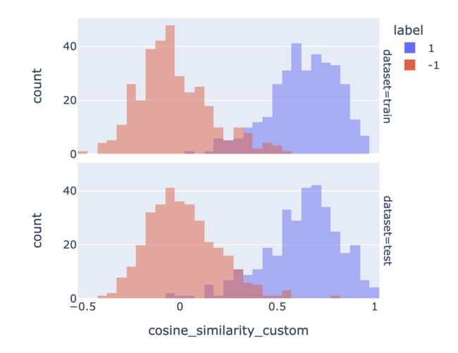
6. 绘制余弦相似度的分布图
在这里,我们使用余弦相似度来衡量文本的相似性。根据我们的经验,大多数距离函数(L1、L2、余弦相似度)的效果都差不多。请注意,我们的嵌入已经被归一化为长度为1,因此余弦相似度等同于点积。
这些图表展示了相似和不相似对的余弦相似度分布之间的重叠程度。如果存在很高程度的重叠,这意味着有些不相似的对具有比某些相似对更大的余弦相似度。
我计算的准确率是一个简单规则的准确率,该规则在余弦相似度高于某个阈值X时预测为“相似(1)”,否则预测为“不相似(0)”。
# 计算在相似度大于x时预测标签为1的准确率(以及其标准误差)
# x通过从-1到1以0.01的步长进行扫描来进行优化
def accuracy_and_se(cosine_similarity: float, labeled_similarity: int) -> Tuple[float]:
    accuracies = []  # 存储准确率的列表
    for threshold_thousandths in range(-1000, 1000, 1):  # 以千分之一为单位从-1000到1000进行循环
        threshold = threshold_thousandths / 1000  # 将千分之一转换为实际阈值
        total = 0  # 总数
        correct = 0  # 正确的数量
        for cs, ls in zip(cosine_similarity, labeled_similarity):  # 对相似度和标签进行迭代
            total += 1  # 总数加1
            if cs > threshold:  # 如果相似度大于阈值
                prediction = 1  # 预测为1
            else:
                prediction = -1  # 预测为-1
            if prediction == ls:  # 如果预测结果与实际标签相同
                correct += 1  # 正确数量加1
        accuracy = correct / total  # 计算准确率
        accuracies.append(accuracy)  # 将准确率添加到列表中
    a = max(accuracies)  # 取最大的准确率
    n = len(cosine_similarity)  # 相似度列表的长度
    standard_error = (a * (1 - a) / n) ** 0.5  # 二项式的标准误差
    return a, standard_error  # 返回准确率和标准误差


# 检查训练集和测试集是否平衡
px.histogram(
    df,
    x="cosine_similarity",
    color="label",
    barmode="overlay",
    width=500,
    facet_row="dataset",
).show()

for dataset in ["train", "test"]:  # 对训练集和测试集进行迭代
    data = df[df["dataset"] == dataset]  # 获取特定数据集的数据
    a, se = accuracy_and_se(data["cosine_similarity"], data["label"])  # 调用accuracy_and_se函数计算准确率和标准误差
    print(f"{dataset} accuracy: {a:0.1%} ± {1.96 * se:0.1%}")  # 打印准确率和标准误差

train accuracy: 89.1% ± 2.4%
test accuracy: 88.8% ± 2.4%
7. 使用提供的训练数据优化矩阵。
# 定义函数embedding_multiplied_by_matrix
# 输入参数为embedding(列表类型)和matrix(torch.tensor类型)
# 将embedding转换为torch.tensor类型,并转换为float类型
# 将embedding与matrix相乘得到modified_embedding
# 将modified_embedding转换为numpy数组类型
# 返回modified_embedding

# 定义函数apply_matrix_to_embeddings_dataframe
# 输入参数为matrix(torch.tensor类型)和df(pd.DataFrame类型)
# 遍历["text_1_embedding", "text_2_embedding"]中的每一列
# 对于每一列,将df[column]中的每个元素应用函数embedding_multiplied_by_matrix,并将结果赋值给df[f"{column}_custom"]
# 对于df中的每一行,计算"cosine_similarity_custom",使用函数cosine_similarity计算"text_1_embedding_custom"和"text_2_embedding_custom"之间的余弦相似度
# 将计算结果赋值给df["cosine_similarity_custom"]
def embedding_multiplied_by_matrix(
    embedding: List[float], matrix: torch.tensor
) -> np.array:
    embedding_tensor = torch.tensor(embedding).float()
    modified_embedding = embedding_tensor @ matrix
    modified_embedding = modified_embedding.detach().numpy()
    return modified_embedding


# compute custom embeddings and new cosine similarities
def apply_matrix_to_embeddings_dataframe(matrix: torch.tensor, df: pd.DataFrame):
    for column in ["text_1_embedding", "text_2_embedding"]:
        df[f"{column}_custom"] = df[column].apply(
            lambda x: embedding_multiplied_by_matrix(x, matrix)
        )
    df["cosine_similarity_custom"] = df.apply(
        lambda row: cosine_similarity(
            row["text_1_embedding_custom"], row["text_2_embedding_custom"]
        ),
        axis=1,
    )
def optimize_matrix(
    modified_embedding_length: int = 2048,  # 在我的简短实验中,更大的值效果更好(2048是巴贝奇编码的长度)
    batch_size: int = 100,
    max_epochs: int = 100,
    learning_rate: float = 100.0,  # 学习率最好与批量大小相似 - 可以尝试一系列值
    dropout_fraction: float = 0.0,  # 在我的测试中,dropout可以提高几个百分点(绝对不是必需的)
    df: pd.DataFrame = df,
    print_progress: bool = True,
    save_results: bool = True,
) -> torch.tensor:
    """返回经过训练数据优化的矩阵"""
    run_id = random.randint(0, 2 ** 31 - 1)  # (范围是任意的)

    # 将数据框转换为torch张量
    # e表示嵌入,s表示相似性标签
    def tensors_from_dataframe(
        df: pd.DataFrame,
        embedding_column_1: str,
        embedding_column_2: str,
        similarity_label_column: str,
    ) -> Tuple[torch.tensor]:
        e1 = np.stack(np.array(df[embedding_column_1].values))
        e2 = np.stack(np.array(df[embedding_column_2].values))
        s = np.stack(np.array(df[similarity_label_column].astype("float").values))

        e1 = torch.from_numpy(e1).float()
        e2 = torch.from_numpy(e2).float()
        s = torch.from_numpy(s).float()

        return e1, e2, s

    # 从数据框中获取训练集和测试集的张量
    e1_train, e2_train, s_train = tensors_from_dataframe(
        df[df["dataset"] == "train"], "text_1_embedding", "text_2_embedding", "label"
    )
    e1_test, e2_test, s_test = tensors_from_dataframe(
        df[df["dataset"] == "test"], "text_1_embedding", "text_2_embedding", "label"
    )

    # 创建数据集和加载器
    dataset = torch.utils.data.TensorDataset(e1_train, e2_train, s_train)
    train_loader = torch.utils.data.DataLoader(
        dataset, batch_size=batch_size, shuffle=True
    )

    # 定义模型(投影嵌入的相似性)
    def model(embedding_1, embedding_2, matrix, dropout_fraction=dropout_fraction):
        e1 = torch.nn.functional.dropout(embedding_1, p=dropout_fraction)
        e2 = torch.nn.functional.dropout(embedding_2, p=dropout_fraction)
        modified_embedding_1 = e1 @ matrix  # @是矩阵乘法
        modified_embedding_2 = e2 @ matrix
        similarity = torch.nn.functional.cosine_similarity(
            modified_embedding_1, modified_embedding_2
        )
        return similarity

    # 定义损失函数
    def mse_loss(predictions, targets):
        difference = predictions - targets
        return torch.sum(difference * difference) / difference.numel()

    # 初始化投影矩阵
    embedding_length = len(df["text_1_embedding"].values[0])
    matrix = torch.randn(
        embedding_length, modified_embedding_length, requires_grad=True
    )

    epochs, types, losses, accuracies, matrices = [], [], [], [], []
    for epoch in range(1, 1 + max_epochs):
        # 遍历训练数据加载器
        for a, b, actual_similarity in train_loader:
            # 生成预测
            predicted_similarity = model(a, b, matrix)
            # 获取损失并进行反向传播
            loss = mse_loss(predicted_similarity, actual_similarity)
            loss.backward()
            # 更新权重
            with torch.no_grad():
                matrix -= matrix.grad * learning_rate
                # 将梯度设置为零
                matrix.grad.zero_()
        # 计算测试损失
        test_predictions = model(e1_test, e2_test, matrix)
        test_loss = mse_loss(test_predictions, s_test)

        # 计算自定义嵌入和新余弦相似度
        apply_matrix_to_embeddings_dataframe(matrix, df)

        # 计算测试准确率
        for dataset in ["train", "test"]:
            data = df[df["dataset"] == dataset]
            a, se = accuracy_and_se(data["cosine_similarity_custom"], data["label"])

            # 记录每个时期的结果
            epochs.append(epoch)
            types.append(dataset)
            losses.append(loss.item() if dataset == "train" else test_loss.item())
            accuracies.append(a)
            matrices.append(matrix.detach().numpy())

            # 可选地打印准确率
            if print_progress is True:
                print(
                    f"Epoch {epoch}/{max_epochs}: {dataset} accuracy: {a:0.1%} ± {1.96 * se:0.1%}"
                )

    data = pd.DataFrame(
        {"epoch": epochs, "type": types, "loss": losses, "accuracy": accuracies}
    )
    data["run_id"] = run_id
    data["modified_embedding_length"] = modified_embedding_length
    data["batch_size"] = batch_size
    data["max_epochs"] = max_epochs
    data["learning_rate"] = learning_rate
    data["dropout_fraction"] = dropout_fraction
    data[
        "matrix"
    ] = matrices  # 保存每个矩阵可能会变得很大;可以随意删除/更改
    if save_results is True:
        data.to_csv(f"{run_id}_optimization_results.csv", index=False)

    return data
# 示例超参数搜索
# 我建议在最初探索时将max_epochs设置为10
results = []  # 创建一个空列表用于存储结果
max_epochs = 30  # 设置最大迭代次数为30
dropout_fraction = 0.2  # 设置dropout比例为0.2

# 针对不同的batch_size和learning_rate进行循环
for batch_size, learning_rate in [(10, 10), (100, 100), (1000, 1000)]:
    # 调用optimize_matrix函数进行矩阵优化,并传入相应的参数
    result = optimize_matrix(
        batch_size=batch_size,
        learning_rate=learning_rate,
        max_epochs=max_epochs,
        dropout_fraction=dropout_fraction,
        save_results=False,
    )
    # 将结果添加到results列表中
    results.append(result)
Epoch 1/30: train accuracy: 89.1% ± 2.4%
Epoch 1/30: test accuracy: 88.4% ± 2.4%
Epoch 2/30: train accuracy: 89.5% ± 2.3%
Epoch 2/30: test accuracy: 88.8% ± 2.4%
Epoch 3/30: train accuracy: 90.6% ± 2.2%
Epoch 3/30: test accuracy: 89.3% ± 2.3%
Epoch 4/30: train accuracy: 91.2% ± 2.2%
Epoch 4/30: test accuracy: 89.7% ± 2.3%
Epoch 5/30: train accuracy: 91.5% ± 2.1%
Epoch 5/30: test accuracy: 90.0% ± 2.3%
Epoch 6/30: train accuracy: 91.9% ± 2.1%
Epoch 6/30: test accuracy: 90.4% ± 2.2%
Epoch 7/30: train accuracy: 92.2% ± 2.0%
Epoch 7/30: test accuracy: 90.7% ± 2.2%
Epoch 8/30: train accuracy: 92.7% ± 2.0%
Epoch 8/30: test accuracy: 90.9% ± 2.2%
Epoch 9/30: train accuracy: 92.7% ± 2.0%
Epoch 9/30: test accuracy: 91.0% ± 2.2%
Epoch 10/30: train accuracy: 93.0% ± 1.9%
Epoch 10/30: test accuracy: 91.6% ± 2.1%
Epoch 11/30: train accuracy: 93.1% ± 1.9%
Epoch 11/30: test accuracy: 91.8% ± 2.1%
Epoch 12/30: train accuracy: 93.4% ± 1.9%
Epoch 12/30: test accuracy: 92.1% ± 2.0%
Epoch 13/30: train accuracy: 93.6% ± 1.9%
Epoch 13/30: test accuracy: 92.4% ± 2.0%
Epoch 14/30: train accuracy: 93.7% ± 1.8%
Epoch 14/30: test accuracy: 92.7% ± 2.0%
Epoch 15/30: train accuracy: 93.7% ± 1.8%
Epoch 15/30: test accuracy: 92.7% ± 2.0%
Epoch 16/30: train accuracy: 94.0% ± 1.8%
Epoch 16/30: test accuracy: 93.0% ± 1.9%
Epoch 17/30: train accuracy: 94.0% ± 1.8%
Epoch 17/30: test accuracy: 93.0% ± 1.9%
Epoch 18/30: train accuracy: 94.2% ± 1.8%
Epoch 18/30: test accuracy: 93.1% ± 1.9%
Epoch 19/30: train accuracy: 94.2% ± 1.8%
Epoch 19/30: test accuracy: 93.1% ± 1.9%
Epoch 20/30: train accuracy: 94.3% ± 1.8%
Epoch 20/30: test accuracy: 93.0% ± 1.9%
Epoch 21/30: train accuracy: 94.5% ± 1.7%
Epoch 21/30: test accuracy: 93.1% ± 1.9%
Epoch 22/30: train accuracy: 94.5% ± 1.7%
Epoch 22/30: test accuracy: 93.3% ± 1.9%
Epoch 23/30: train accuracy: 94.6% ± 1.7%
Epoch 23/30: test accuracy: 93.3% ± 1.9%
Epoch 24/30: train accuracy: 94.6% ± 1.7%
Epoch 24/30: test accuracy: 93.3% ± 1.9%
Epoch 25/30: train accuracy: 94.8% ± 1.7%
Epoch 25/30: test accuracy: 93.3% ± 1.9%
Epoch 26/30: train accuracy: 94.8% ± 1.7%
Epoch 26/30: test accuracy: 93.4% ± 1.9%
Epoch 27/30: train accuracy: 94.8% ± 1.7%
Epoch 27/30: test accuracy: 93.4% ± 1.9%
Epoch 28/30: train accuracy: 94.9% ± 1.7%
Epoch 28/30: test accuracy: 93.4% ± 1.9%
Epoch 29/30: train accuracy: 94.9% ± 1.7%
Epoch 29/30: test accuracy: 93.4% ± 1.9%
Epoch 30/30: train accuracy: 94.9% ± 1.7%
Epoch 30/30: test accuracy: 93.3% ± 1.9%
Epoch 1/30: train accuracy: 89.7% ± 2.3%
Epoch 1/30: test accuracy: 89.1% ± 2.4%
Epoch 2/30: train accuracy: 89.8% ± 2.3%
Epoch 2/30: test accuracy: 89.9% ± 2.3%
Epoch 3/30: train accuracy: 90.3% ± 2.2%
Epoch 3/30: test accuracy: 90.0% ± 2.3%
Epoch 4/30: train accuracy: 91.0% ± 2.2%
Epoch 4/30: test accuracy: 90.3% ± 2.2%
Epoch 5/30: train accuracy: 91.3% ± 2.1%
Epoch 5/30: test accuracy: 90.3% ± 2.2%
Epoch 6/30: train accuracy: 91.8% ± 2.1%
Epoch 6/30: test accuracy: 90.4% ± 2.2%
Epoch 7/30: train accuracy: 92.4% ± 2.0%
Epoch 7/30: test accuracy: 91.0% ± 2.2%
Epoch 8/30: train accuracy: 92.8% ± 2.0%
Epoch 8/30: test accuracy: 91.3% ± 2.1%
Epoch 9/30: train accuracy: 93.1% ± 1.9%
Epoch 9/30: test accuracy: 91.6% ± 2.1%
Epoch 10/30: train accuracy: 93.4% ± 1.9%
Epoch 10/30: test accuracy: 91.9% ± 2.1%
Epoch 11/30: train accuracy: 93.4% ± 1.9%
Epoch 11/30: test accuracy: 91.8% ± 2.1%
Epoch 12/30: train accuracy: 93.6% ± 1.9%
Epoch 12/30: test accuracy: 92.1% ± 2.0%
Epoch 13/30: train accuracy: 93.7% ± 1.8%
Epoch 13/30: test accuracy: 92.4% ± 2.0%
Epoch 14/30: train accuracy: 93.7% ± 1.8%
Epoch 14/30: test accuracy: 92.5% ± 2.0%
Epoch 15/30: train accuracy: 93.9% ± 1.8%
Epoch 15/30: test accuracy: 92.8% ± 2.0%
Epoch 16/30: train accuracy: 94.0% ± 1.8%
Epoch 16/30: test accuracy: 92.8% ± 2.0%
Epoch 17/30: train accuracy: 94.0% ± 1.8%
Epoch 17/30: test accuracy: 92.8% ± 2.0%
Epoch 18/30: train accuracy: 94.2% ± 1.8%
Epoch 18/30: test accuracy: 92.8% ± 2.0%
Epoch 19/30: train accuracy: 94.2% ± 1.8%
Epoch 19/30: test accuracy: 92.8% ± 2.0%
Epoch 20/30: train accuracy: 94.2% ± 1.8%
Epoch 20/30: test accuracy: 93.1% ± 1.9%
Epoch 21/30: train accuracy: 94.3% ± 1.8%
Epoch 21/30: test accuracy: 93.3% ± 1.9%
Epoch 22/30: train accuracy: 94.3% ± 1.8%
Epoch 22/30: test accuracy: 93.3% ± 1.9%
Epoch 23/30: train accuracy: 94.5% ± 1.7%
Epoch 23/30: test accuracy: 93.3% ± 1.9%
Epoch 24/30: train accuracy: 94.5% ± 1.7%
Epoch 24/30: test accuracy: 93.3% ± 1.9%
Epoch 25/30: train accuracy: 94.6% ± 1.7%
Epoch 25/30: test accuracy: 93.4% ± 1.9%
Epoch 26/30: train accuracy: 94.6% ± 1.7%
Epoch 26/30: test accuracy: 93.3% ± 1.9%
Epoch 27/30: train accuracy: 94.6% ± 1.7%
Epoch 27/30: test accuracy: 93.4% ± 1.9%
Epoch 28/30: train accuracy: 94.8% ± 1.7%
Epoch 28/30: test accuracy: 93.4% ± 1.9%
Epoch 29/30: train accuracy: 94.8% ± 1.7%
Epoch 29/30: test accuracy: 93.3% ± 1.9%
Epoch 30/30: train accuracy: 94.8% ± 1.7%
Epoch 30/30: test accuracy: 93.4% ± 1.9%
Epoch 1/30: train accuracy: 90.7% ± 2.2%
Epoch 1/30: test accuracy: 89.9% ± 2.3%
Epoch 2/30: train accuracy: 90.9% ± 2.2%
Epoch 2/30: test accuracy: 90.3% ± 2.2%
Epoch 3/30: train accuracy: 91.6% ± 2.1%
Epoch 3/30: test accuracy: 90.3% ± 2.2%
Epoch 4/30: train accuracy: 92.2% ± 2.0%
Epoch 4/30: test accuracy: 90.7% ± 2.2%
Epoch 5/30: train accuracy: 92.4% ± 2.0%
Epoch 5/30: test accuracy: 91.3% ± 2.1%
Epoch 6/30: train accuracy: 92.5% ± 2.0%
Epoch 6/30: test accuracy: 91.8% ± 2.1%
Epoch 7/30: train accuracy: 93.0% ± 1.9%
Epoch 7/30: test accuracy: 92.2% ± 2.0%
Epoch 8/30: train accuracy: 93.1% ± 1.9%
Epoch 8/30: test accuracy: 92.7% ± 2.0%
Epoch 9/30: train accuracy: 93.3% ± 1.9%
Epoch 9/30: test accuracy: 92.5% ± 2.0%
Epoch 10/30: train accuracy: 93.4% ± 1.9%
Epoch 10/30: test accuracy: 92.7% ± 2.0%
Epoch 11/30: train accuracy: 93.6% ± 1.9%
Epoch 11/30: test accuracy: 92.8% ± 2.0%
Epoch 12/30: train accuracy: 93.7% ± 1.8%
Epoch 12/30: test accuracy: 92.8% ± 2.0%
Epoch 13/30: train accuracy: 94.0% ± 1.8%
Epoch 13/30: test accuracy: 93.0% ± 1.9%
Epoch 14/30: train accuracy: 93.9% ± 1.8%
Epoch 14/30: test accuracy: 93.0% ± 1.9%
Epoch 15/30: train accuracy: 94.2% ± 1.8%
Epoch 15/30: test accuracy: 93.0% ± 1.9%
Epoch 16/30: train accuracy: 94.2% ± 1.8%
Epoch 16/30: test accuracy: 93.0% ± 1.9%
Epoch 17/30: train accuracy: 94.3% ± 1.8%
Epoch 17/30: test accuracy: 93.0% ± 1.9%
Epoch 18/30: train accuracy: 94.5% ± 1.7%
Epoch 18/30: test accuracy: 93.1% ± 1.9%
Epoch 19/30: train accuracy: 94.5% ± 1.7%
Epoch 19/30: test accuracy: 93.1% ± 1.9%
Epoch 20/30: train accuracy: 94.6% ± 1.7%
Epoch 20/30: test accuracy: 93.3% ± 1.9%
Epoch 21/30: train accuracy: 94.8% ± 1.7%
Epoch 21/30: test accuracy: 93.3% ± 1.9%
Epoch 22/30: train accuracy: 94.8% ± 1.7%
Epoch 22/30: test accuracy: 93.4% ± 1.9%
Epoch 23/30: train accuracy: 94.8% ± 1.7%
Epoch 23/30: test accuracy: 93.4% ± 1.9%
Epoch 24/30: train accuracy: 94.8% ± 1.7%
Epoch 24/30: test accuracy: 93.4% ± 1.9%
Epoch 25/30: train accuracy: 94.8% ± 1.7%
Epoch 25/30: test accuracy: 93.4% ± 1.9%
Epoch 26/30: train accuracy: 94.9% ± 1.7%
Epoch 26/30: test accuracy: 93.6% ± 1.9%
Epoch 27/30: train accuracy: 94.9% ± 1.7%
Epoch 27/30: test accuracy: 93.6% ± 1.9%
Epoch 28/30: train accuracy: 94.9% ± 1.7%
Epoch 28/30: test accuracy: 93.6% ± 1.9%
Epoch 29/30: train accuracy: 95.1% ± 1.6%
Epoch 29/30: test accuracy: 93.6% ± 1.9%
Epoch 30/30: train accuracy: 95.1% ± 1.6%
Epoch 30/30: test accuracy: 93.6% ± 1.9%
# 将所有结果合并为一个DataFrame
runs_df = pd.concat(results)
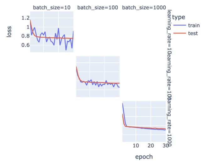
# 绘制训练损失和测试损失随时间的变化图
px.line(
runs_df, # 数据源为合并后的DataFrame
line_group="run_id", # 按照run_id分组,每个run_id对应一条线
x="epoch", # x轴为epoch
y="loss", # y轴为loss
color="type", # 根据type进行颜色区分
hover_data=["batch_size", "learning_rate", "dropout_fraction"], # 鼠标悬停时显示的额外信息
facet_row="learning_rate", # 按照learning_rate进行行分面
facet_col="batch_size", # 按照batch_size进行列分面
width=500, # 图的宽度
).show() # 显示图像
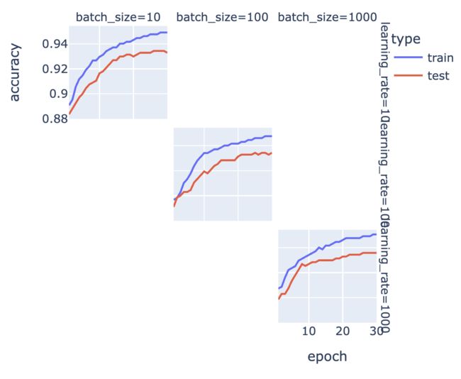
# 绘制准确率随时间的变化图
px.line(
runs_df, # 数据源为合并后的DataFrame
line_group="run_id", # 按照run_id分组,每个run_id对应一条线
x="epoch", # x轴为epoch
y="accuracy", # y轴为accuracy
color="type", # 根据type进行颜色区分
hover_data=["batch_size", "learning_rate", "dropout_fraction"], # 鼠标悬停时显示的额外信息
facet_row="learning_rate", # 按照learning_rate进行行分面
facet_col="batch_size", # 按照batch_size进行列分面
width=500, # 图的宽度
).show() # 显示图像
8. 绘制训练期间找到的最佳矩阵的前后对比图,展示结果
矩阵越好,它就能更清晰地分离相似和不相似的对。
# 从所有运行结果中找到准确率最高的一组
best_run = runs_df.sort_values(by="accuracy", ascending=False).iloc[0]
# 获取最佳运行结果对应的矩阵
best_matrix = best_run["matrix"]
# 将最佳矩阵应用到原始数据中的嵌入向量上
apply_matrix_to_embeddings_dataframe(best_matrix, df)
# 绘制自定义前的相似度分布图
px.histogram(
    df,  # 数据框
    x="cosine_similarity",  # x轴为"cosine_similarity"列的值
    color="label",  # 颜色按"label"列的值分组
    barmode="overlay",  # 设置柱状图的叠加模式
    width=500,  # 设置图表宽度为500
    facet_row="dataset",  # 按"dataset"列的值分行显示子图
).show()  # 显示图表

# 从数据框中筛选出"dataset"列为"test"的数据
test_df = df[df["dataset"] == "test"]
# 计算测试集的准确率和标准误差
a, se = accuracy_and_se(test_df["cosine_similarity"], test_df["label"])
# 打印测试集的准确率和标准误差
print(f"Test accuracy: {a:0.1%} ± {1.96 * se:0.1%}")

# 绘制自定义后的相似度分布图
px.histogram(
    df,  # 数据框
    x="cosine_similarity_custom",  # x轴为"cosine_similarity_custom"列的值
    color="label",  # 颜色按"label"列的值分组
    barmode="overlay",  # 设置柱状图的叠加模式
    width=500,  # 设置图表宽度为500
    facet_row="dataset",  # 按"dataset"列的值分行显示子图
).show()  # 显示图表

# 计算自定义后的测试集准确率和标准误差
a, se = accuracy_and_se(test_df["cosine_similarity_custom"], test_df["label"])
# 打印自定义后的测试集准确率和标准误差
print(f"Test accuracy after customization: {a:0.1%} ± {1.96 * se:0.1%}")

Test accuracy: 88.8% ± 2.4%
Test accuracy after customization: 93.6% ± 1.9%
# 定义变量best_matrix,用于乘以嵌入向量
best_matrix  # 这是可以用来乘以嵌入向量的最佳矩阵
array([[-1.2566795e+00, -1.5297449e+00, -1.3271648e-01, ...,
        -1.2859761e+00, -5.3254390e-01,  4.8364732e-01],
       [-1.4826347e+00,  9.2656955e-02, -4.2437232e-01, ...,
         1.1872858e+00, -1.0831847e+00, -1.0683593e+00],
       [-2.2029283e+00, -1.9703420e+00,  3.1125939e-01, ...,
         2.2947595e+00,  5.5780332e-03, -6.0171342e-01],
       ...,
       [-1.1019799e-01,  1.3599515e+00, -4.7677776e-01, ...,
         6.5626711e-01,  7.2359240e-01,  3.0733588e+00],
       [ 1.6624762e-03,  4.2648423e-01, -1.1380885e+00, ...,
         8.7202555e-01,  9.3173909e-01, -1.6760436e+00],
       [ 7.7449006e-01,  4.9213606e-01,  3.5407653e-01, ...,
         1.3460466e+00, -1.9509128e-01,  7.7514690e-01]], dtype=float32)