R: Introduction to the Tidyverse
1. data wrangling
library(gapminder) /*加载数据集*/
library(dplyr)
gapminder /*check the dataset*/
The filter verb
# Single condition
gapminder %>%
    filter(year == 1957)
# Multiple conditions
gapminder %>%
    filter(year == 2002, country == "China")
* note: %>% take whatever is before it, and feed it in the next steps
The arrange verb
arrange sorts the observations in a dataset, in ascending or descending order based on one of its variables
# Sort in ascending order of lifeExp
gapminder %>%
    arrange(lifeExp)
# Sort in descending order of lifeExp
gapminder %>%
    arrange(desc(lifeExp))
The mutate verb
gapminder %>%
    mutate(lifeExpMonths = 12 * lifeExp)
Combine the verbs
# Filter, mutate, and arrange the gapminder dataset
gapminder %>%
    filter(year == 2007) %>%
    mutate(lifeExpMonths = 12 * lifeExp) %>%
    arrange(desc(lifeExpMonths))
2. data visualization
1) assign the variable
创建筛选后的新变量
# Create gapminder_1952
gapminder_1952 <- gapminder %>%
    filter(year == 1952)
2) create a scatter plot
ggplot(gapminder_1952, aes(x = pop, y = gdpPercap)) +
  geom_point()
3) log scales
图像变形,log转换
ggplot(gapminder_1952, aes(x = pop, y = lifeExp)) +
  geom_point() +
  scale_x_log10()
4) additional aesthetics (size, color)
为小类添加颜色, 标识点的大小
ggplot(gapminder_1952, aes(x = pop, y = lifeExp, size = gdpPercap, color = continent)) +
  geom_point() +
  scale_x_log10()
5) faceting
facet can visualize subgroup
ggplot(gapminder_1952, aes(x = pop, y = lifeExp)) +
  geom_point() +
  facet_wrap(~ continent) +
  scale_x_log10()
按照大洲进行可视化,如图:

Take another example,
ggplot(gapminder, aes(x = gdpPercap, y = lifeExp, color = continent, size = pop)) +
    geom_point() +
    scale_x_log10() +
    facet_wrap(~year)
如图

3. grouping and summarizing
1) summarize()
e.g. calculate the median life expectancy into a column
gapminder %>%
  filter(year == 1957) %>%
  summarize(medianLifeExp = median(lifeExp))
e.g. two orders in summarize()
gapminder %>%
    filter(year == 1957) %>%
    summarize(medianLifeExp = median(lifeExp), maxGdpPercap = max(gdpPercap))
2) The group_by verb
可以用于分组总结
gapminder %>%
    filter(year == 1957) %>%
    group_by(continent) %>%
    summarize(medianLifeEXP = median(lifeExp), maxGdpPercap = max(gdpPercap))
3) visualizing over time
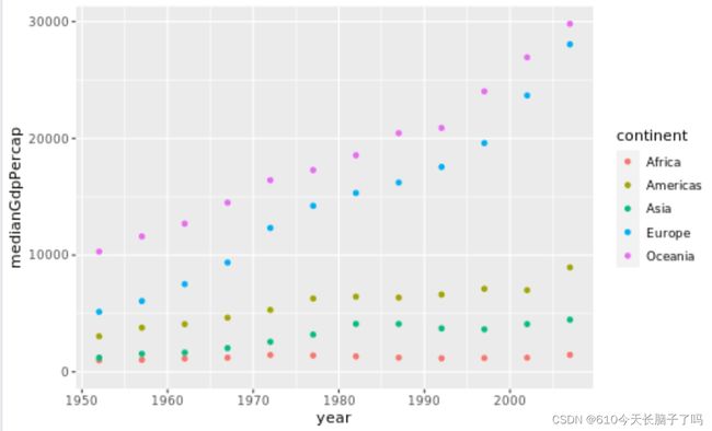
# Summarize medianGdpPercap within each continent within each year: by_year_continent
by_year_continent <- gapminder %>%
  group_by(continent, year) %>%
  summarize(medianGdpPercap = median(gdpPercap))

# Plot the change in medianGdpPercap in each continent over time
ggplot(by_year_continent, aes(x = year, y = medianGdpPercap, color = continent)) +
  geom_point() +
  expand_limits(y = 0)
note:
expand_limits(y=0): y-axis starts at zero
如图
4. types of visualization
4.1 line plot
geom_line()
# Summarize the median gdpPercap by year, then save it as by_year
by_year <- gapminder %>%
    group_by(year) %>%
    summarize(medianGdpPercap=median(gdpPercap))

# Create a line plot showing the change in medianGdpPercap over time
ggplot(by_year, aes(x=year, y=medianGdpPercap)) +
    geom_line() +
    expand_limits(y=0)
4.2 bar plot
geom_col()
# Create a bar plot showing medianGdp by continent
ggplot(by_continent, aes(x=continent, medianGdpPercap)) +
    geom_col()
4.3 histograms
geom_histogram()
notes: in the bracket, we can add "bins=*number" or "binwidth=*number", etc.
geom_histogram()

gapminder_1952 <- gapminder %>%

  filter(year == 1952)

# Create a histogram of population (pop), with x on a log scale

ggplot(gapminder_1952, aes(x=pop)) +

  geom_histogram() +

  scale_x_log10()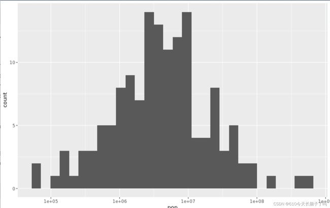
4.4 boxplots
geom_boxplot()
gapminder_1952 <- gapminder %>%
  filter(year == 1952)

# Create a boxplot comparing gdpPercap among continents
ggplot(gapminder_1952, aes(x=continent, y=gdpPercap)) +
  geom_boxplot() +
  scale_y_log10()
4.5 other details
1) add a title to the graph
+ ggtitle(" *title ")