C语言数字图像处理(十):Otus算法,移动平均和区域生长算法
0. 前言
这是C语言数字图像处理系列的最后一章。作为这个博客帐户的第一个系列和作品,很高兴看到了一百多位新增的粉丝,也非常感谢大家在这两周陪伴!
这个系列的内容来自博主在香港学习计算机科学时候的一门课程,这是一门本科生和研究生都可以选修的课。也就是说,如果读者能够学习和实践这10章里面的内容,在有需要的时候配合教科书(数字图像处理 (第三版),作者: Rafael C. Gonzalez)加深理解,那么你就对DIP里面所有常用的算法有了一个比较全面的掌握。
再次,如果你喜欢这个系列的文章或者感觉对你有帮助,请帮忙给我的仓库点一个⭐️!
仓库地址和这一章节的所有代码都在:10. Otus, Moving Average, and Region Growing
再次感谢!
1. Otus算法
以下是Otus的算法执行步骤:
(1) 计算输入图像的归一化直方图,使用![]() 来表示直方图的每个组成部分。 其中
来表示直方图的每个组成部分。 其中 是强度为 的像素数。
(2)计算 = 0,1,2, ... , − 1 的累积和 ![]() :
:

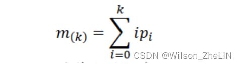
(3) 计算 = 0,1,2, ... , − 1 的累积平均值 ():
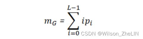
(5)计算全局强度的平均值:
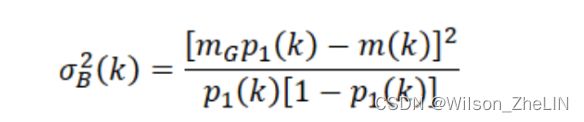
(5) 计算 = 0,1,2, ... , − 1 的类间方差 ![]() :
:
(6)获取最佳阈值*,如果最大值不唯一,则使用对应检测到的最大值的平均值得到*:

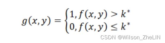
(7)二值化:
图像和结果对比 (arge_septagon_gaussian_noise_mean_0_std_50_added.pgm):
![]()
结果分析:
从结果来看,Otus算法的分割效果比之前的全局阈值算法要好很多。 Otsu算法衡量最优分割阈值的标准是类间方差最大,当类间方差最大时为最优。 但该算法对噪声和目标尺寸非常敏感,需要进行降噪处理才能取得可观的效果。
代码实现(更完整的代码见顶部GitHub):
1. Otus算法:
unsigned char* Otsu_Algorithm(unsigned char *tempin, int width, int height) {
    unsigned char *tempout;
    int size = width * height;
    tempout = (unsigned char *) malloc(size);
    float histogram[256], ratio[256], sigma[256];

    for(int i = 0; i < 256; i++) {
        histogram[i] = 0;
    }
    for(int i = 0; i < size; i++) {
        int temp = tempin[i];
        histogram[temp] += 1;
    }
    for(int i = 0; i < 256; i++) {
        ratio[i] = histogram[i] / (float)size;
    }

    float mg = sum(256, ratio);

    for(int i = 0; i < 256; i++) {
        sigma[i] = calculate_sigma(i, mg, ratio);
    }

    float max = sigma[0];
    int max_count = 1, k = 0;
    for(int i = 1; i < 256; i++) {
        if(abs(sigma[i] - max) < 1e-10) {
            k += i;
            max_count++;
        }
        else if(sigma[i] > max) {
            max = sigma[i];
            max_count = 1;
            k = i;
        }
    }
    float k_final = (float)k / (float)max_count;

    for(int i = 0; i < size; i++) {
        if(tempin[i] <= k_final) tempout[i] = 0;
        else tempout[i] = 255;
    }
    return tempout;
}
(2)计算sigma函数和sum函数:
float calculate_sigma(int k, float mg, float ratio[]){
    float p1k = 0.0;
    for(int i = 0; i < k; i++) {
        p1k += ratio[i];
    }
    float mk = sum(k, ratio);
    if(p1k < 1e-10 || (1 - p1k) < 1e-10) return 0.0;
    else return pow(mg * p1k - mk, 2) / (p1k * (1 - p1k));
}
2. 分区Otus算法
将图像划分为不重叠的矩形,以保证每个矩形的光照近似均匀,然后对每个矩形分别进行Otus算法。 Otus算法与上述第1部分相同。
图像和结果对比 (septagon_noisy_shaded.pgm):

结果分析:
分区Otus的方法属于变量阈值法。 因为噪声和均匀照明对阈值算法的性能起着重要作用。 例如,在我们这次使用带光照变化的图像中,全局 Otus 的分割存在比较明显的问题。尽管原始图像被分成了6部分,但是结果仍然存在一些很小误差,因为直方图中有两种模式,并且两种模式都有明显的波谷。因此,当对象和背景占据相当大小的区域时,分区分割的效果更好。 但如果图像仅仅包含物体或仅仅包含背景则会失效。
代码实现:
void Otsu_Partition(Image *image) {
    unsigned char *tempin, *tempout;
    int y = (float)image->Height / 2.0 + 1;
    int x = (float)image->Width / 3.0 + 1;
    int size_partition = x * y;
    Image *outimage;
    outimage = CreateNewImage(image, (char*)"#testing Function");
    tempin = image->data;
    tempout = outimage->data;
    unsigned char inPart1[size_partition], inPart2[size_partition], inPart3[size_partition], inPart4[size_partition], inPart5[size_partition], inPart6[size_partition];
    unsigned char *outPart1, *outPart2, *outPart3, *outPart4, *outPart5, *outPart6;

    for(int i = 0; i < image->Height; i++) {
        for(int j = 0; j < image->Width; j++){
            if(j - 2*x >= 0 && i - y >= 0) {
                inPart6[x * (i-y) + (j-2*x)] = tempin[image->Width * i + j];
            }
            else if(j - x < 0 && i - y < 0) {
                inPart1[x * i + j] = tempin[image->Width * i + j];
            }
            else if(j - 2*x >= 0 && i - y < 0) {
                inPart3[x * i + (j-2*x)] = tempin[image->Width * i + j];
            }
            else if(j - x < 0 && i - y >= 0) {
                inPart4[x * (i-y) + j] = tempin[image->Width * i + j];
            }
            else if(j >= x && j < 2*x && i - y >= 0) {
                inPart5[x * (i-y) + (j-x)] = tempin[image->Width * i + j];
            }
            else if(j >= x && j < 2*x && i - y < 0) {
                inPart2[x * i + (j-x)] = tempin[image->Width * i + j];
            }
        }
    }

    outPart1 = Otsu_Algorithm(inPart1, x, y);
    outPart2 = Otsu_Algorithm(inPart2, x, y);
    outPart3 = Otsu_Algorithm(inPart3, x, y);
    outPart4 = Otsu_Algorithm(inPart4, x, y);
    outPart5 = Otsu_Algorithm(inPart5, x, y);
    outPart6 = Otsu_Algorithm(inPart6, x, y);

    for(int i = 0; i < image->Height; i++) {
        for(int j = 0; j < image->Width; j++){
            if(j - 2*x >= 0 && i - y >= 0) {
                tempout[image->Width * i + j] = outPart6[x * (i-y) + (j-2*x)];
            }
            else if(j - x < 0 && i - y < 0) {
                tempout[image->Width * i + j] = outPart1[x * i + j];
            }
            else if(j - 2*x >= 0 && i - y < 0) {
                tempout[image->Width * i + j] = outPart3[x * i + (j-2*x)];
            }
            else if(j - x < 0 && i - y >= 0) {
                tempout[image->Width * i + j] = outPart4[x * (i-y) + j];
            }
            else if(j >= x && j < 2*x && i - y >= 0) {
                tempout[image->Width * i + j] = outPart5[x * (i-y) + (j-x)];
            }
            else if(j >= x && j < 2*x && i - y < 0) {
                tempout[image->Width * i + j] = outPart2[x * i + (j-x)];
            }
        }
    }
    SavePNMImage(outimage, (char*)"Otsu_Partition.pgm");
}
3. 移动平均阈值算法
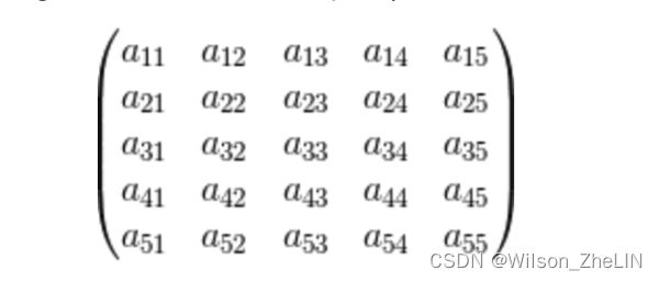
假设有一个 5x5 的图像,如下所示, 代表 (, ) 处的强度。
然后再进行往复形线性扫描(zigzag linear scan),因此需要将二维矩阵转为一维行矩阵,顺序如下:
![]()
之后,我们在数组的开头插入 个零来计算每个点的平均值:
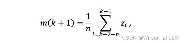
其中是用于计算平均值的点数,索引之外的任何位置都将被视为0。然后我们得到分割阈值:
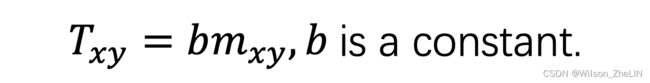
其中 b 是一个常数。最后对图像进行二值化以获得结果。
图像和结果对比 (Moving_Average.pgm):

结果分析:
移动平均法是一种可变阈值处理方法。这种方法以之字形线性扫描整个图像,目的是减少图像中光照的偏差。这解决了全局阈值无法处理的光强变化问题。通常来说,当对象和图像的尺寸相对较小或较薄时,如被斑点遮挡的文本图像或正弦波形的亮度,该算法效果较好。
代码实现(更完整的代码见顶部GitHub):
Z = (unsigned char *) malloc(size+20);

for(int i = 0; i < 20; i++) {
    Z[i] = 0;
}

int index = 20;
for(int i = 0; i < image->Height; i++) {
    for(int j = 0; j < image->Width; j++){
        Z[index++] = tempin[image->Width * i + j];
    }
    i++;
    for(int j = image->Width-1; j <= 0; j++){
        Z[index++] = tempin[image->Width * i + j];
    }
}

for(int i = 0; i < size; i++) {
    float sum = 0.0;
    for(int j = 0; j < 20; j++) {
        sum += Z[i-j+20];
    }
    T[i] = sum / 20.0 * 0.5;
}

index = 0;
for(int i = 0; i < image->Height; i++) {
    for(int j = 0; j < image->Width; j++){
        T_inverse[index++] = T[image->Width * i + j];
    }
    i++;
    for(int j = image->Width-1; j <= 0; j++){
        T_inverse[index++] = T[image->Width * i + j];
    }
}

for(int i = 0; i < size; i++) {
    if(tempin[i] > T_inverse[i]) tempout[i] = 255;
    else tempout[i] = 0;
}
4. 区域生长算法:
我的区域生长算法实现步骤如下:
1)计算图像中各个强度的直方图
2)将5%强度最高的像素作为“种子”并标记
3)以每个种子为中心,考虑8个邻居像素,如果满足增长标准(大于设定强度或差值足够小),则标记邻居有效像素
4)重复步骤3,直到遍历完图像中的每个点,生长结束。
此外,我的算法中加入了深度优先搜索。 所以我的程序的时间复杂度将是(_),因为图像中的每个像素只需要遍历和标记一次。
图像和结果对比 (defective_weld.pgm,noisy_region.pgm):

结果分析:
区域生长法是一种将像素或子区域根据预定义的标准聚集成更大区域的过程。其基本思想是从一组生长点开始,将与生长点具有相似属性的相邻像素或区域合并。
区域生长的优点包括:
- 可以对具有相同特征的连通区域进行分割
- 能够提供良好的边界信息和分割结果
- 在生长过程中可以自由指定生长标准,同时可以选择多个标准
其缺点包括:
- 计算成本高(通过深度优先搜索算法解决)
- 噪声和强度不均匀性可能导致孔洞和过度分割
- 对图像中的阴影处理效果不佳
代码实现:
void region_growing(Image *image) {
    unsigned char *tempin, *tempout1, *tempout2;
    Image *outimage1, *outimage2;
    int size = image->Width * image->Height;
    int checkBoard[size];
    float histogram[256];
    outimage1 = CreateNewImage(image, (char*)"#testing Function");
    outimage2 = CreateNewImage(image, (char*)"#testing Function");
    tempin = image->data;
    tempout1 = outimage1->data;
    tempout2 = outimage2->data;

    for(int i = 0; i < 256; i++) {
        histogram[i] = 0;
    }
    for(int i = 0; i < size; i++) {
        int temp = tempin[i];
        histogram[temp] += 1;
    }

    int T = 256;
    int light_count = 0;
    while(light_count < (float)size * 0.004) {
        T--;
        light_count += histogram[T];
    }
    for(int i = 0; i < size; i++) {
        if(tempin[i] >= T) tempout1[i] = 255;
        else tempout1[i] = 0;
    }
    SavePNMImage(outimage1, (char*)"connected.pgm");

    for(int i = 0; i < size; i++) {
        if(tempout1[i] == 255) checkBoard[i] = 1;
        else checkBoard[i] = 2;
    }
    for(int i = 0; i < image->Height; i++) {
        for(int j = 0; j < image->Width; j++){
            DFS_MarkPixels(image, checkBoard, j, i);
        }
    }

    for(int i = 0; i < size; i++) {
        if(checkBoard[i] == 3) tempout2[i] = 255;
        else tempout2[i] = 0;
    }
    SavePNMImage(outimage2, (char*)"Region_growing.pgm");
}
5. 结束语
恭喜,至此,你已经走完了数字图像处理全部的章节。感谢所有读者的支持和相伴。
非常希望你能够帮我的仓库点一个星,仓库地址和这一章节的代码:GitHub
期待再见!
-END-