CIFAR 10实现图像分类反卷积特张图可视化

from keras.datasets import cifar10

from keras import regularizers
from keras.callbacks import ModelCheckpoint
from keras.layers import Conv2D, Activation, BatchNormalization, MaxPooling2D, Dropout, Flatten, Dense
from keras.models import Sequential
from keras.preprocessing.image import ImageDataGenerator
from matplotlib import pyplot
from keras import optimizers
import numpy as np

# download and split the data
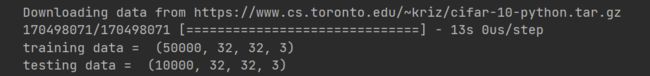
(x_train, y_train), (x_test, y_test) = cifar10.load_data()
x_train = x_train.astype('float32')
x_test = x_test.astype('float32')

print("training data = ", x_train.shape)
print("testing data = ", x_test.shape)

# Normalize the data to speed up training
mean = np.mean(x_train)
std = np.std(x_train)
x_train = (x_train-mean)/(std+1e-7)
x_test = (x_test-mean)/(std+1e-7)

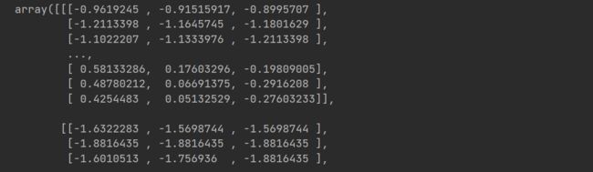
# let's look at the normalized values of a sample image
x_train[0]

# one-hot encode the labels in train and test datasets
# we use “to_categorical” function in keras
from keras.utils import to_categorical
num_classes = 10
y_train = to_categorical(y_train,num_classes)
y_test = to_categorical(y_test,num_classes)

# let's display one of the one-hot encoded labels
y_train[0]

from keras.layers import Conv2DTranspose
# build the model

# number of hidden units variable
# we are declaring this variable here and use it in our CONV layers to make it easier to update from one place
base_hidden_units = 32

# l2 regularization hyperparameter
weight_decay = 1e-4

# instantiate an empty sequential model
model = Sequential()

# CONV1
# notice that we defined the input_shape here because this is the first CONV layer.
# we don’t need to do that for the remaining layers
model.add(Conv2D(base_hidden_units, (3,3), padding='same', kernel_regularizer=regularizers.l2(weight_decay), input_shape=x_train.shape[1:]))
model.add(Activation('relu'))
model.add(BatchNormalization())

# CONV2
model.add(Conv2D(base_hidden_units, (3,3), padding='same', kernel_regularizer=regularizers.l2(weight_decay)))
model.add(Activation('relu'))
model.add(BatchNormalization())
model.add(MaxPooling2D(pool_size=(2,2)))
model.add(Dropout(0.2))

# CONV2反卷积层
model.add(Conv2DTranspose(base_hidden_units, (2, 2), strides=(2, 2), padding='same'))
model.add(Activation('relu'))
model.add(BatchNormalization())

# CONV3
model.add(Conv2D(2*base_hidden_units, (3,3), padding='same', kernel_regularizer=regularizers.l2(weight_decay)))
model.add(Activation('relu'))
model.add(BatchNormalization())

# CONV4
model.add(Conv2D(2*base_hidden_units, (3,3), padding='same', kernel_regularizer=regularizers.l2(weight_decay)))
model.add(Activation('relu'))
model.add(BatchNormalization())
model.add(MaxPooling2D(pool_size=(2,2)))
model.add(Dropout(0.3))

# CONV4反卷积
model.add(Conv2DTranspose(2*base_hidden_units, (2, 2), strides=(2, 2), padding='same'))
model.add(Activation('relu'))
model.add(BatchNormalization())

# CONV5
model.add(Conv2D(4*base_hidden_units, (3,3), padding='same', kernel_regularizer=regularizers.l2(weight_decay)))
model.add(Activation('relu'))
model.add(BatchNormalization())

# CONV6
model.add(Conv2D(4*base_hidden_units, (3,3), padding='same', kernel_regularizer=regularizers.l2(weight_decay)))
model.add(Activation('relu'))
model.add(BatchNormalization())
model.add(MaxPooling2D(pool_size=(2,2)))
model.add(Dropout(0.4))

# FC7
model.add(Flatten())
model.add(Dense(num_classes, activation='softmax'))

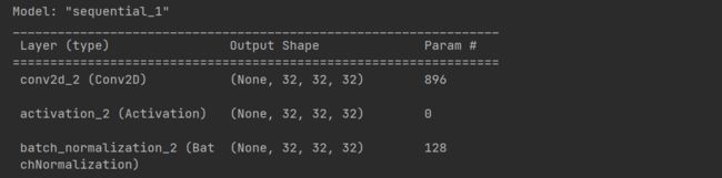
# print model summary
model.summary()

# data augmentation
datagen = ImageDataGenerator(
    rotation_range=15,
    width_shift_range=0.1,
    height_shift_range=0.1,
    horizontal_flip=True,
    vertical_flip=False
    )

# compute the data augmentation on the training set
datagen.fit(x_train)

# training
from tensorflow.keras.optimizers import legacy
batch_size = 256
epochs=5
# 200
checkpointer = ModelCheckpoint(filepath='model.125epochs.hdf5', verbose=1, save_best_only=True)

# you can try any of these optimizers by uncommenting the line
#optimizer = rmsprop(lr=0.001,decay=1e-6)
optimizer = legacy.Adam(learning_rate=0.001,decay=1e-6)

#optimizer =keras.optimizers.rmsprop(lr=0.0003,decay=1e-6)
model.compile(loss='categorical_crossentropy', optimizer=optimizer, metrics=['accuracy'])
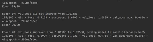
history = model.fit(datagen.flow(x_train, y_train, batch_size=batch_size), callbacks=[checkpointer],
                steps_per_epoch=x_train.shape[0] // batch_size, epochs=epochs,verbose=2,
                validation_data=(x_test,y_test))

# evaluating the model
scores = model.evaluate(x_test, y_test, batch_size=128, verbose=1)
print('\nTest result: %.3f loss: %.3f' % (scores[1]*100,scores[0]))

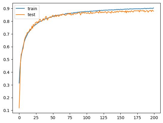
# plot learning curves of model accuracy

pyplot.plot(history.history['accuracy'], label='train')
pyplot.plot(history.history['val_accuracy'], label='test')
pyplot.legend()
pyplot.show()

from keras.models import Model

# 提取特定图层的特征图
layer_name = 'conv2d_2'  # 将其更改为所需的图层名称
intermediate_layer_model = Model(inputs=model.input,
                                 outputs=model.get_layer(layer_name).output)

# 从数据集中选择图像
sample_image = x_train[0]  # 将其更改为所需的图像

# 重塑图像以匹配模型输入的形状
sample_image = sample_image.reshape((1,) + sample_image.shape)

# 获取所选图像的中间输出（特征图
feature_maps = intermediate_layer_model.predict(sample_image)

# 可视化
import matplotlib.pyplot as plt

# 假设特征地图的形状为 (1、高、宽、过滤器数量)
num_filters = feature_maps.shape[-1]
fig, axes = plt.subplots(1, num_filters, figsize=(20, 2))

for i in range(num_filters):
    axes[i].imshow(feature_maps[0, :, :, i], cmap='viridis')
    axes[i].axis('off')

plt.show()