- 基于蜣螂算法优化多头注意力机制的卷积神经网络结合双向长短记忆神经网络实现温度预测DBO-CNN-biLSTM-Multihead-Attention附matlab代码
matlab科研助手
神经网络算法cnn
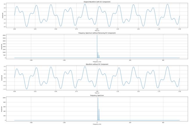
✅作者简介:热爱科研的Matlab仿真开发者,修心和技术同步精进,代码获取、论文复现及科研仿真合作可私信。个人主页:Matlab科研工作室个人信条:格物致知。更多Matlab完整代码及仿真定制内容点击智能优化算法神经网络预测雷达通信无线传感器电力系统信号处理图像处理路径规划元胞自动机无人机物理应用机器学习内容介绍温度预测在气象学、农业、能源等领域具有重要的应用价值。随着大数据和人工智能技术的快速发
- 股票基金量化开源平台对比
Mr.小海
开源开源金融
股票基金量化开源平台对比分析报告引言研究背景与意义在金融科技快速发展的背景下,量化交易已成为现代金融市场中投资者追求高效与精准交易的核心工具。通过程序化方式,投资者能够迅速处理海量市场数据,制定并执行复杂交易策略,其高效性、低情绪干扰及策略多样性等优势显著[1]。特别是随着人工智能技术的深化,2025年基于深度学习与机器学习的开源量化工具持续涌现,推动行业向数据驱动转型——量化交易将决策逻辑从经验
- 开源基金/股票量化平台调研报告
Mr.小海
金融
开源基金/股票量化平台调研报告引言调研背景与目的近年来,随着人工智能技术的持续深化,量化交易领域迎来了深刻变革。2025年,基于深度学习和机器学习的开源工具不断涌现,不仅在技术层面实现突破,更在实际应用中展现出强大竞争优势,推动行业创新与升级[1].作为融合数学、统计与计算机技术的科技驱动型金融策略,量化交易通过自动化与数据驱动方法提升投资决策效率与准确性,已成为金融机构与投资者追求超额收益的重要
- 同步发电机与逆变型电源故障电流特性对比实验研究
神经网络15044
MATLAB专栏仿真模型生成对抗网络学习人工智能开发语言matlab
同步发电机与逆变型电源故障电流特性对比实验研究前些天发现了一个巨牛的人工智能学习网站,通俗易懂,风趣幽默,忍不住分享一下给大家。点击跳转到网站。1.研究背景与意义随着可再生能源在电力系统中的渗透率不断提高,逆变型电源(Inverter-BasedResources,IBR)在电网中的比重日益增加。与传统同步发电机相比,IBR的故障响应特性存在显著差异,这对电力系统的保护设计和运行控制提出了新的挑战
- AIGC革命:基于魔搭社区的LLM应用开发实战——从模型微调到系统部署
Liudef06小白
AIGC人工智能特殊专栏人工智能魔搭AIGCLLM
AIGC革命:基于魔搭社区的LLM应用开发实战——从模型微调到系统部署1.AIGC技术演进与魔搭社区生态解析人工智能生成内容(AIGC)正在重塑内容创作、软件开发和人机交互的边界。从OpenAI的GPT系列到StabilityAI的StableDiffusion,生成式AI技术正以惊人的速度发展。在这场技术革命中,魔搭社区(ModelScope)作为中国领先的AI模型开源平台,正成为开发者探索AI
- 人工智能界的“黑话“大揭秘:AI新词汇速成指南
人工智能界的"黑话"大揭秘:AI新词汇速成指南你是否曾在科技大佬们讨论AI时一头雾水?听到RAG、Agent、PromptEngineering时以为他们在说天书?别担心,今天我们就来一场AI术语的"通俗化运动",让你轻松混入AI圈子,秒变内行人!LLM(大型语言模型):AI界的"大胃王"LLM是吞噬了互联网大部分文字的"数据饕餮"。特点:训练数据以TB(万亿字节)计算参数动辄上千亿计算能力堪比小
- 解密Claude系列:从原理到实践的全方位解析
软考和人工智能学堂
强化学习人工智能Claude快速入门Claude
引言:Claude系列模型的崛起在人工智能领域,大型语言模型(LLM)的发展日新月异。OpenAI的GPT系列和Anthropic的Claude系列无疑是这一领域的双子星。Claude系列模型以其独特的"ConstitutionalAI"理念和强大的对话能力,正在重塑人机交互的未来。本文将深入探讨Claude系列的技术原理、架构特点,并通过实践代码展示其强大能力。Claude系列的技术演进1.Cl
- 元宇宙:中国数字经济的新赛道——基于游戏生态、AI与区块链的创新实践
boyedu
元宇宙域名游戏人工智能区块链元宇宙
引言:数字经济时代的“新大陆”在数字技术的浪潮中,元宇宙正从科幻概念跃升为全球科技竞争的焦点。中国,作为全球数字经济规模第二大的经济体,正以独特的路径探索元宇宙的发展——以游戏生态为起点,融合人工智能(AI)与区块链技术,构建一个虚实融合的数字新世界。这一路径不仅契合中国在5G、AI、区块链等领域的技术积累,更与“数字经济”“新质生产力”等国家战略形成共振。本文将从技术融合、经济价值、社会影响三个
- 智能体架构设计的五大核心原则:构建下一代AI系统的工程基石
一休哥助手
人工智能
引言:智能体架构的范式演进人工智能领域正经历从孤立模型向自主智能体的范式转变。2025年,全球AI智能体市场规模突破200亿美元,在金融、医疗、制造等领域的渗透率超40%。然而,智能体开发仍面临协作效率低(多智能体任务重叠率达30%)、安全风险高(工具调用错误率18%)和系统僵化(需求变更迭代周期超2周)三大痛点。本文基于产业实践提炼五大核心设计原则,为构建下一代智能体系统提供架构指南。传统LLM
- 昇思MindSpore创新训练营·长三角站开始报名!
昇思MindSpore
人工智能自然语言处理深度学习
一、介绍为充分发挥长三角研究型大学联盟教学实践基地共建共享功能,加强华东高校优秀青年学子的交流与互动,提供学生与产业界接触的机会,上海交通大学与华为技术有限公司共同发起,面向长三角研究型大学学生开设昇思MindSpore创新训练营。本次训练营以实践项目和业界需求为牵引,以学生实践为主线,让学生在实践的过程中学习和实践人工智能相关知识,掌握相关技术和工具,紧跟业界最新趋势,加深对人工智能行业的认识,
- OPPO未来科技大会,科技感满满!你最爱哪些黑科技呢?
冬天不冷了
#OPPO未来科技大会#OPPO携手IHSMarkit发布《智能互融:借助5G、人工智能和云技术,释放机遇》白皮书,表明人工智能、云技术和边缘设备、互联和物联网的协同努力,将为企业和消费者带来价值。看了一下早上的,是说明年绿厂要发不少好玩的产品,比如智能手表AR眼镜之类的,有些可能跟Reno3一块发,对外是说构建生态万物互联,其实就是多卖几样多赚钱,然后用这钱砸了搞技术赚更大的钱,毕竟现场说了未来
- 2025年最流行跑分最高的图片理解大模型调研报告
2025年最流行跑分最高的图片理解大模型调研报告引言当前,图片理解大模型正处于快速演进阶段,其技术发展呈现多维度深化与融合的特征。从技术演进方向来看,多模态融合已成为核心趋势之一,文本、图像、视频等不同模态的交互与协同能力显著提升。大型视觉-语言模型(LVLMs)作为人工智能领域的重要突破,标志着多模态理解与交互进入变革性发展阶段,尽管当前模型在各类任务中表现出色,但在细粒度视觉任务等基础能力层面
- 基于DTLC-AEC与DTLN的轻量级实时语音增强系统设计与实现
神经网络15044
仿真模型神经网络机器学习图像处理cnn人工智能机器人
基于DTLC-AEC与DTLN的轻量级实时语音增强系统设计与实现前些天发现了一个巨牛的人工智能学习网站,通俗易懂,风趣幽默,忍不住分享一下给大家。点击跳转到网站。1.引言在当今的互联网通信时代,实时语音通信已成为人们日常生活中不可或缺的一部分。然而,语音通信质量常常受到回声、背景噪声等因素的严重影响。为了解决这些问题,我们需要高效的语音增强技术。本文将详细介绍如何将DTLC-AEC(深度学习回声消
- 第 20 课时:GPU 管理和 Device Plugin 工作机制(车漾)
阿里云云原生
CNCFX阿里巴巴云原生技术公开课阿里云KubernetesCNCF专家团队CNCF专家团队CNCF专家团队Kubernetes
本文将主要分享以下几个方面的内容:需求来源GPU的容器化Kubernetes的GPU管理工作原理课后思考与实践需求来源2016年,随着AlphaGo的走红和TensorFlow项目的异军突起,一场名为AI的技术革命迅速从学术圈蔓延到了工业界,所谓AI革命从此拉开了帷幕。经过三年的发展,AI有了许许多多的落地场景,包括智能客服、人脸识别、机器翻译、以图搜图等功能。其实机器学习或者说是人工智能,并不是
- 智慧后厨检测算法构建智能厨房防护网
智驱力人工智能
人工智能算法高温预警行为识别口罩识别食品安全手套识别
智慧后厨检测:构建安全洁净厨房的智能解决方案背景:传统后厨管理的痛点与智慧化需求餐饮行业后厨管理长期面临操作规范难落实、安全隐患难察觉、卫生状况难追溯等痛点。传统人工巡检效率低、覆盖面有限,难以实现24小时无死角监管。例如,厨师未佩戴口罩或手套、违规使用手机、动火离人等行为,可能引发食品安全事故或火灾风险。随着人工智能技术的成熟,智慧后厨检测系统通过集成多种算法,实现了对后厨人员行为、环境卫生、设
- 《Python Web 框架深度剖析:Django、Flask 与 FastAPI 的选择之道》
清水白石008
课程教程学习笔记开发语言python前端django
《PythonWeb框架深度剖析:Django、Flask与FastAPI的选择之道》开篇引入:从“胶水语言”到Web架构核心Python,自1991年由GuidovanRossum发布以来,凭借其简洁优雅的语法和强大的生态系统,逐渐成为全球最受欢迎的编程语言之一。它不仅在数据科学、人工智能、自动化脚本等领域大放异彩,更在Web开发领域构建起一套成熟的技术体系。作为一位长期从事Python开发与教
- 【DeepSeek实战】10、模型上下文协议(MCP)全解析:从核心架构到实战应用,揭秘AI协作的“凤雏”之力
无心水
人工智能架构DeepSeek实战模型上下文协议MCPCSDN技术干货DeepSeekAI大模型
在人工智能技术飞速发展的今天,大型语言模型(LLM)的能力不断突破,但跨模型协作、上下文一致性维护等问题却成为制约AI系统向更智能、更协同方向发展的瓶颈。模型上下文协议(ModelContextProtocol,MCP)作为专为大模型设计的标准化通信框架,如同“凤雏”之于“卧龙”,为解决这些核心问题提供了关键方案。本文将全面解析MCP的核心概念、架构设计、实操代码、应用案例及未来趋势,通过5000
- AI交互的初期魅力与后期维护挑战
AI交互的初期魅力与后期维护挑战引言在当今数字化时代,人工智能(AI)技术正迅速渗透到各个领域,特别是人机交互方面。许多开发者、设计师和用户在初次与AI交互时,往往感受到一种“一时爽”的快感。这种交互方式看似高效、智能,能够快速响应需求,提供即时反馈。然而,随着时间的推移,这种初期魅力往往会转化为高昂的后期维护成本。本文将深入讨论AI交互的这一双面性,重点分析细节沟通不足以及UI设计中AI难以处理
- 【云原生】Helm来管理Kubernetes集群的详细使用方法与综合应用实战
景天科技苑
云原生K8S零基础到进阶实战云原生kubernetes容器Helmk8sk8s集群
✨✨欢迎大家来到景天科技苑✨✨养成好习惯,先赞后看哦~作者简介:景天科技苑《头衔》:大厂架构师,华为云开发者社区专家博主,阿里云开发者社区专家博主,CSDN全栈领域优质创作者,掘金优秀博主,51CTO博客专家等。《博客》:Python全栈,前后端开发,小程序开发,人工智能,js逆向,App逆向,网络系统安全,数据分析,Django,fastapi,flask等框架,云原生k8s,linux,she
- Transformer:自注意力驱动的神经网络革命引擎
大千AI助手
人工智能Python#OTHERtransformer神经网络深度学习google人工智能机器学习大模型
本文由「大千AI助手」原创发布,专注用真话讲AI,回归技术本质。拒绝神话或妖魔化。搜索「大千AI助手」关注我,一起撕掉过度包装,学习真实的AI技术!从语言理解到多模态智能的通用架构基石⚙️一、核心定义与历史意义Transformer是由Google团队在2017年论文《AttentionIsAllYouNeed》中提出的深度学习架构,其颠覆性创新在于:完全摒弃RNN/CNN:仅依赖自注意力机制(S
- Python面向对象编程(OOP)详解:通俗易懂的全面指南
盛夏绽放
python开发语言有问必答
前些天发现了一个巨牛的人工智能学习网站,通俗易懂,风趣幽默,忍不住分享一下给大家。点击跳转到网站。文章目录Python面向对象编程(OOP)详解:通俗易懂的全面指南一、OOP基本概念1.什么是面向对象编程?2.OOP的四大支柱3.核心概念对比表二、类和对象1.类(Class)vs对象(Object)2.类结构详解三、OOP三大特性详解1.封装(Encapsulation)2.继承(Inherita
- 马斯克整出的半仙儿,Chat GPT会让多少白领失业?可能会带来哪些变化?
良辰美景5566
这几天,ChatGPT火了,是美国一家叫OpenAI的高科技公司研发的,背后的投资人是谁?——埃隆马斯克!这哥们儿只要一出手,注定就和新奇呀伟大呀啥的绑在一起了,他搞的项目,比如特斯拉、星链、脑机接口,光听名字就透着不俗。很多人纳闷儿,他这次搞得ChatGPT是个啥玩意儿?简单说就是一个人工智能聊天软件,这个软件比以往的智能聊天软件强在哪儿?这么说吧,这简直就是个半仙儿啊。如果您是一位老人,这个C
- 量子计算与AI融合的技术突破与实践路径
量子计算与人工智能的融合正开启一个全新的技术纪元,这种"量智融合"不是简单的技术叠加,而是多领域、多学科的横向连接,通过协同创新实现非线性增长。本文将深入探讨这一领域的最新进展、技术实现路径以及行业应用案例。电子-光子-量子一体化芯片:硬件基础突破2025年7月,美国波士顿大学、加州大学伯克利分校和西北大学团队联合开发出全球首个电子-光子-量子一体化芯片系统。这一突破性成果发表在《自然·电子学》杂
- 117、Python机器学习:数据预处理与特征工程技巧
多多的编程笔记
python机器学习开发语言
Python开发之机器学习准备:数据预处理与特征工程机器学习是当前人工智能领域的热门方向之一。而作为机器学习的核心组成部分,数据预处理与特征工程对于模型的性能有着至关重要的影响。本文将带领大家了解数据预处理与特征工程的基本概念,以及它们在实际应用场景中的重要性。数据预处理数据预处理是机器学习中的第一步,它的主要目的是将原始数据转换成适合进行机器学习模型训练的形式。就像我们在做饭之前需要清洗和准备食
- 2025年各细分产业链企业数据(汽车、数字经济、食品、制造业)
经管数据库
汽车智能手机数据分析
本数据包含2025年及之前的所有上中下游企业信息,67个细分产业。汽车专区、数字经济专区、数字创意专区、未来产业专区、高端装备专区、新能源专区、食品农业专区、传统制造业专区等71个文件。汽车专区:充电桩制造动力电池汽车材料制造汽车制造汽车制造设备汽车座椅制造驱动电机制造燃料电池汽车制造燃料电池系统制造新能源汽车制造智能驾驶智能视觉数字经济专区:5g边缘计算大数据类服务器光通信集成电路区块链人工智能
- 2024年,想要靠做软件测试获得高薪,还有机会吗?
朱公子的Note
软件测试
2024年,科技行业风云变幻,随着自动化技术和人工智能的发展,软件测试领域的竞争愈发激烈。很多人会问,现在还投身软件测试,真的能拿到高薪吗?尤其是当越来越多的自动化工具涌现,手动测试员会不会被淘汰?时间过得真快,一眨眼,2024年已经过去了一大半。最近正值金九银十招聘季,后台不免又出现了这几个同学们关心的问题:2024年还能转行软件测试吗?零基础转行可行吗?那么,2024年,软件测试行业的高薪岗位
- 2023-09-15 五角大楼探索生成式人工智能解决方案
泰格
佳文砺道智库2023-09-1409:58发表于北京据“防务头条”网9月12日报道,美国研究机构“特殊竞争力研究项目”(SCSP)的一份报称告,如果美国想在制定生成式人工智能的开发和使用规范方面引领全球,就必须增加联邦研发支出,建立新的政府机构,或者改变现有的政府机构。生成式人工智能可以加速新药和网络安全解决方案的发现,从根本上实现更好的计算机网络,并提高公众的理解。但在对手手中,它可能会导致更多
- 人工智能服务器处理器的全新定义 两大头部品牌旗舰款的王者之争!云储存cpu_云服务器处理器_企业服务器处理器
一、旗舰处理器架构解析IntelXeon6900系列代表着英特尔在服务器处理器领域的最新成果,采用增强版Intel7制程工艺打造。该系列最高配置56个物理核心,通过超线程技术支持112个逻辑线程,在处理多线程任务时展现出卓越的性能表现。内存子系统方面,支持8通道DDR5-4800内存配置,最高可扩展至4TB容量,为内存密集型应用提供了充足带宽。特别值得一提的是其集成的AMX高级矩阵扩展指令集,这项
- 院级医疗AI管理流程—基于数据共享、算法开发与工具链治理的系统化框架
Allen_Lyb
医疗高效编程研发人工智能算法时序数据库经验分享健康医疗
医疗AI:从“单打独斗”到“协同共进”在科技飞速发展的今天,医疗人工智能(AI)正以前所未有的速度改变着传统医疗模式。从最初在影像诊断、临床决策支持、药物发现等单一领域的“单点突破”,医疗AI如今已迈向“系统级协同”的新阶段。曾经,医疗AI的应用多集中在某一特定环节,比如利用深度学习算法分析医学影像,辅助医生进行疾病诊断。这种单点突破式的应用虽然在一定程度上提高了医疗效率,但随着医疗行业对AI技术
- python--自动化的机器学习(AutoML)
Q_ytsup5681
python自动化机器学习
自动化机器学习(AutoML)是一种将自动化技术应用于机器学习模型开发流程的方法,旨在简化或去除需要专业知识的复杂步骤,让非专家用户也能轻松创建和部署机器学习模型**[^3^]。具体介绍如下:1.自动化的概念:自动化是指使设备在无人或少量人参与的情况下完成一系列任务的过程。这一概念随着电子计算机的发明和发展而不断进化,从最初的物理机械到后来的数字程序控制,再到现在的人工智能和机器学习,自动化已经渗
- apache 安装linux windows
墙头上一根草
apacheinuxwindows
linux安装Apache 有两种方式一种是手动安装通过二进制的文件进行安装,另外一种就是通过yum 安装,此中安装方式,需要物理机联网。以下分别介绍两种的安装方式
通过二进制文件安装Apache需要的软件有apr,apr-util,pcre
1,安装 apr 下载地址:htt
- fill_parent、wrap_content和match_parent的区别
Cb123456
match_parentfill_parent
fill_parent、wrap_content和match_parent的区别:
1)fill_parent
设置一个构件的布局为fill_parent将强制性地使构件扩展,以填充布局单元内尽可能多的空间。这跟Windows控件的dockstyle属性大体一致。设置一个顶部布局或控件为fill_parent将强制性让它布满整个屏幕。
2) wrap_conte
- 网页自适应设计
天子之骄
htmlcss响应式设计页面自适应
网页自适应设计
网页对浏览器窗口的自适应支持变得越来越重要了。自适应响应设计更是异常火爆。再加上移动端的崛起,更是如日中天。以前为了适应不同屏幕分布率和浏览器窗口的扩大和缩小,需要设计几套css样式,用js脚本判断窗口大小,选择加载。结构臃肿,加载负担较大。现笔者经过一定时间的学习,有所心得,故分享于此,加强交流,共同进步。同时希望对大家有所
- [sql server] 分组取最大最小常用sql
一炮送你回车库
SQL Server
--分组取最大最小常用sql--测试环境if OBJECT_ID('tb') is not null drop table tb;gocreate table tb( col1 int, col2 int, Fcount int)insert into tbselect 11,20,1 union allselect 11,22,1 union allselect 1
- ImageIO写图片输出到硬盘
3213213333332132
javaimage
package awt;
import java.awt.Color;
import java.awt.Font;
import java.awt.Graphics;
import java.awt.image.BufferedImage;
import java.io.File;
import java.io.IOException;
import javax.imagei
- 自己的String动态数组
宝剑锋梅花香
java动态数组数组
数组还是好说,学过一两门编程语言的就知道,需要注意的是数组声明时需要把大小给它定下来,比如声明一个字符串类型的数组:String str[]=new String[10]; 但是问题就来了,每次都是大小确定的数组,我需要数组大小不固定随时变化怎么办呢? 动态数组就这样应运而生,龙哥给我们讲的是自己用代码写动态数组,并非用的ArrayList 看看字符
- pinyin4j工具类
darkranger
.net
pinyin4j工具类Java工具类 2010-04-24 00:47:00 阅读69 评论0 字号:大中小
引入pinyin4j-2.5.0.jar包:
pinyin4j是一个功能强悍的汉语拼音工具包,主要是从汉语获取各种格式和需求的拼音,功能强悍,下面看看如何使用pinyin4j。
本人以前用AscII编码提取工具,效果不理想,现在用pinyin4j简单实现了一个。功能还不是很完美,
- StarUML学习笔记----基本概念
aijuans
UML建模
介绍StarUML的基本概念,这些都是有效运用StarUML?所需要的。包括对模型、视图、图、项目、单元、方法、框架、模型块及其差异以及UML轮廓。
模型、视与图(Model, View and Diagram)
&
- Activiti最终总结
avords
Activiti id 工作流
1、流程定义ID:ProcessDefinitionId,当定义一个流程就会产生。
2、流程实例ID:ProcessInstanceId,当开始一个具体的流程时就会产生,也就是不同的流程实例ID可能有相同的流程定义ID。
3、TaskId,每一个userTask都会有一个Id这个是存在于流程实例上的。
4、TaskDefinitionKey和(ActivityImpl activityId
- 从省市区多重级联想到的,react和jquery的差别
bee1314
jqueryUIreact
在我们的前端项目里经常会用到级联的select,比如省市区这样。通常这种级联大多是动态的。比如先加载了省,点击省加载市,点击市加载区。然后数据通常ajax返回。如果没有数据则说明到了叶子节点。 针对这种场景,如果我们使用jquery来实现,要考虑很多的问题,数据部分,以及大量的dom操作。比如这个页面上显示了某个区,这时候我切换省,要把市重新初始化数据,然后区域的部分要从页面
- Eclipse快捷键大全
bijian1013
javaeclipse快捷键
Ctrl+1 快速修复(最经典的快捷键,就不用多说了)Ctrl+D: 删除当前行 Ctrl+Alt+↓ 复制当前行到下一行(复制增加)Ctrl+Alt+↑ 复制当前行到上一行(复制增加)Alt+↓ 当前行和下面一行交互位置(特别实用,可以省去先剪切,再粘贴了)Alt+↑ 当前行和上面一行交互位置(同上)Alt+← 前一个编辑的页面Alt+→ 下一个编辑的页面(当然是针对上面那条来说了)Alt+En
- js 笔记 函数
征客丶
JavaScript
一、函数的使用
1.1、定义函数变量
var vName = funcation(params){
}
1.2、函数的调用
函数变量的调用: vName(params);
函数定义时自发调用:(function(params){})(params);
1.3、函数中变量赋值
var a = 'a';
var ff
- 【Scala四】分析Spark源代码总结的Scala语法二
bit1129
scala
1. Some操作
在下面的代码中,使用了Some操作:if (self.partitioner == Some(partitioner)),那么Some(partitioner)表示什么含义?首先partitioner是方法combineByKey传入的变量,
Some的文档说明:
/** Class `Some[A]` represents existin
- java 匿名内部类
BlueSkator
java匿名内部类
组合优先于继承
Java的匿名类,就是提供了一个快捷方便的手段,令继承关系可以方便地变成组合关系
继承只有一个时候才能用,当你要求子类的实例可以替代父类实例的位置时才可以用继承。
在Java中内部类主要分为成员内部类、局部内部类、匿名内部类、静态内部类。
内部类不是很好理解,但说白了其实也就是一个类中还包含着另外一个类如同一个人是由大脑、肢体、器官等身体结果组成,而内部类相
- 盗版win装在MAC有害发热,苹果的东西不值得买,win应该不用
ljy325
游戏applewindowsXPOS
Mac mini 型号: MC270CH-A RMB:5,688
Apple 对windows的产品支持不好,有以下问题:
1.装完了xp,发现机身很热虽然没有运行任何程序!貌似显卡跑游戏发热一样,按照那样的发热量,那部机子损耗很大,使用寿命受到严重的影响!
2.反观安装了Mac os的展示机,发热量很小,运行了1天温度也没有那么高
&nbs
- 读《研磨设计模式》-代码笔记-生成器模式-Builder
bylijinnan
java设计模式
声明: 本文只为方便我个人查阅和理解,详细的分析以及源代码请移步 原作者的博客http://chjavach.iteye.com/
/**
* 生成器模式的意图在于将一个复杂的构建与其表示相分离,使得同样的构建过程可以创建不同的表示(GoF)
* 个人理解:
* 构建一个复杂的对象,对于创建者(Builder)来说,一是要有数据来源(rawData),二是要返回构
- JIRA与SVN插件安装
chenyu19891124
SVNjira
JIRA安装好后提交代码并要显示在JIRA上,这得需要用SVN的插件才能看见开发人员提交的代码。
1.下载svn与jira插件安装包,解压后在安装包(atlassian-jira-subversion-plugin-0.10.1)
2.解压出来的包里下的lib文件夹下的jar拷贝到(C:\Program Files\Atlassian\JIRA 4.3.4\atlassian-jira\WEB
- 常用数学思想方法
comsci
工作
对于搞工程和技术的朋友来讲,在工作中常常遇到一些实际问题,而采用常规的思维方式无法很好的解决这些问题,那么这个时候我们就需要用数学语言和数学工具,而使用数学工具的前提却是用数学思想的方法来描述问题。。下面转帖几种常用的数学思想方法,仅供学习和参考
函数思想
把某一数学问题用函数表示出来,并且利用函数探究这个问题的一般规律。这是最基本、最常用的数学方法
- pl/sql集合类型
daizj
oracle集合typepl/sql
--集合类型
/*
单行单列的数据,使用标量变量
单行多列数据,使用记录
单列多行数据,使用集合(。。。)
*集合:类似于数组也就是。pl/sql集合类型包括索引表(pl/sql table)、嵌套表(Nested Table)、变长数组(VARRAY)等
*/
/*
--集合方法
&n
- [Ofbiz]ofbiz初用
dinguangx
电商ofbiz
从github下载最新的ofbiz(截止2015-7-13),从源码进行ofbiz的试用
1. 加载测试库
ofbiz内置derby,通过下面的命令初始化测试库
./ant load-demo (与load-seed有一些区别)
2. 启动内置tomcat
./ant start
或
./startofbiz.sh
或
java -jar ofbiz.jar
&
- 结构体中最后一个元素是长度为0的数组
dcj3sjt126com
cgcc
在Linux源代码中,有很多的结构体最后都定义了一个元素个数为0个的数组,如/usr/include/linux/if_pppox.h中有这样一个结构体: struct pppoe_tag { __u16 tag_type; __u16 tag_len; &n
- Linux cp 实现强行覆盖
dcj3sjt126com
linux
发现在Fedora 10 /ubutun 里面用cp -fr src dest,即使加了-f也是不能强行覆盖的,这时怎么回事的呢?一两个文件还好说,就输几个yes吧,但是要是n多文件怎么办,那还不输死人呢?下面提供三种解决办法。 方法一
我们输入alias命令,看看系统给cp起了一个什么别名。
[root@localhost ~]# aliasalias cp=’cp -i’a
- Memcached(一)、HelloWorld
frank1234
memcached
一、简介
高性能的架构离不开缓存,分布式缓存中的佼佼者当属memcached,它通过客户端将不同的key hash到不同的memcached服务器中,而获取的时候也到相同的服务器中获取,由于不需要做集群同步,也就省去了集群间同步的开销和延迟,所以它相对于ehcache等缓存来说能更好的支持分布式应用,具有更强的横向伸缩能力。
二、客户端
选择一个memcached客户端,我这里用的是memc
- Search in Rotated Sorted Array II
hcx2013
search
Follow up for "Search in Rotated Sorted Array":What if duplicates are allowed?
Would this affect the run-time complexity? How and why?
Write a function to determine if a given ta
- Spring4新特性——更好的Java泛型操作API
jinnianshilongnian
spring4generic type
Spring4新特性——泛型限定式依赖注入
Spring4新特性——核心容器的其他改进
Spring4新特性——Web开发的增强
Spring4新特性——集成Bean Validation 1.1(JSR-349)到SpringMVC
Spring4新特性——Groovy Bean定义DSL
Spring4新特性——更好的Java泛型操作API
Spring4新
- CentOS安装JDK
liuxingguome
centos
1、行卸载原来的:
[root@localhost opt]# rpm -qa | grep java
tzdata-java-2014g-1.el6.noarch
java-1.7.0-openjdk-1.7.0.65-2.5.1.2.el6_5.x86_64
java-1.6.0-openjdk-1.6.0.0-11.1.13.4.el6.x86_64
[root@localhost
- 二分搜索专题2-在有序二维数组中搜索一个元素
OpenMind
二维数组算法二分搜索
1,设二维数组p的每行每列都按照下标递增的顺序递增。
用数学语言描述如下:p满足
(1),对任意的x1,x2,y,如果x1<x2,则p(x1,y)<p(x2,y);
(2),对任意的x,y1,y2, 如果y1<y2,则p(x,y1)<p(x,y2);
2,问题:
给定满足1的数组p和一个整数k,求是否存在x0,y0使得p(x0,y0)=k?
3,算法分析:
(
- java 随机数 Math与Random
SaraWon
javaMathRandom
今天需要在程序中产生随机数,知道有两种方法可以使用,但是使用Math和Random的区别还不是特别清楚,看到一篇文章是关于的,觉得写的还挺不错的,原文地址是
http://www.oschina.net/question/157182_45274?sort=default&p=1#answers
产生1到10之间的随机数的两种实现方式:
//Math
Math.roun
- oracle创建表空间
tugn
oracle
create temporary tablespace TXSJ_TEMP
tempfile 'E:\Oracle\oradata\TXSJ_TEMP.dbf'
size 32m
autoextend on
next 32m maxsize 2048m
extent m
- 使用Java8实现自己的个性化搜索引擎
yangshangchuan
javasuperword搜索引擎java8全文检索
需要对249本软件著作实现句子级别全文检索,这些著作均为PDF文件,不使用现有的框架如lucene,自己实现的方法如下:
1、从PDF文件中提取文本,这里的重点是如何最大可能地还原文本。提取之后的文本,一个句子一行保存为文本文件。
2、将所有文本文件合并为一个单一的文本文件,这样,每一个句子就有一个唯一行号。
3、对每一行文本进行分词,建立倒排表,倒排表的格式为:词=包含该词的总行数N=行号