图像恢复及滤波处理
图像恢复及滤波处理
1.基本概念:
a.图像恢复是通过计算机处理,对质量下降的图像加以重建或恢复的处理过程。因摄像机与物体相对运动、系统误差、畸变、噪声等因素的影响,使图像往往不是真实景物的完善映像。在图像恢复中,需建立造成图像质量下降的退化模型,然后运用相反过程来恢复原来图像,并运用一定准则来判定是否得到图像的最佳恢复。在遥感图像处理中,为消除遥感图像的失真、畸变,恢复目标的反射波谱特性和正确的几何位置,通常需要对图像进行恢复处理,包括辐射校正、大气校正、条带噪声消除、几何校正等内容。
b.图像恢复采用的方法:
滤波器被广泛地用于图象的预处理,抑制图象噪声,增强对比度,以及强化图象的边沿特征。运用较为广泛的线性滤波器如平均值滤波器,能较好地抑制图象中的加性噪声。 但是,线性滤波器会引起图象的钝化或模糊,使得图象中物体边界产生位移。特别是,在图象受到乘性噪声或脉冲噪声的干扰,如超声波及雷达成像中普遍存在的斑点噪声,线性滤波器就不能取得预期的效果。中值滤波器,就像其名字一样,是用该像素的相邻像素的灰度中值来代替该像素的值,是一种非线性滤波器。
c.椒盐噪声:噪声脉冲可正可负,正脉冲是以白点(盐点)出现,负脉冲是以黑点(胡椒点)出现。
d.算术均值滤波器和几何均值滤波器(尤其是后者)更适合处理高斯或均匀等随机噪声。
谐波均值滤波器:对于“盐”噪声效果好,不适用“胡椒”噪声,善于处理高斯噪声那样的脉冲噪声。
缺点是:必须知道噪声是暗噪声还是亮噪声,以便选择合适的Q号。
逆谐波均值滤波器:Q为其阶数,当Q为正数,用于消除“胡椒”噪声;当Q为负数,用于消除“盐”噪声;
当Q=0退变为算术均值滤波器,当Q=-1时,退变为谐波均值滤波器。
e.顺序统计滤波器:
中值滤波器:处理脉冲型加性噪声,重复使用中值滤波器处理图像会使图像模糊,尽可能保持希望的处理次数。
最大值:除去图像中的“胡椒”噪声,但是会从黑色物体的边缘移走一些黑色像素。
最大值:除去图像中的“盐”噪声,但是会从白色物体的边缘移走一些白色像素。
修正的阿尔法均值滤波器:d值可以取0到mn-1之间的任意数,当d=0时,退变为算术均值滤波器,
当d=(mn-1)/2退变为中值滤波器,d取其他值时,在包含多种噪声的情况下非常适用。
f.巴特沃斯IIR滤波器的设计:
在MATLAB下,设计巴特沃斯IIR滤波器可使用butter函数。
Butter函数可设计低通、高通、带通和带阻的数字和模拟IIR滤波器,其特性为使通带内的幅度响应最大限度地平坦,但同时损失截止频率处的下降斜度。在期望通带平滑的情况下,可使用butter函数。
butter函数的用法为:[b,a]=butter(n,Wn,/ftype/)
其中n代表滤波器阶数,Wn代表滤波器的截止频率,这两个参数可使用buttord函数来确定。buttord函数可在给定滤波器性能的情况下,求出巴特沃斯滤波器的最小阶数n,同时给出对应的截止频率Wn。
buttord函数的用法为:[n,Wn]= buttord(Wp,Ws,Rp,Rs)
其中Wp和Ws分别是通带和阻带的拐角频率(截止频率),其取值范围为0至1之间。当其值为1时代表采样频率的一半。Rp和Rs分别是通带和阻带区的波纹系数。
g.不同类型(高通、低通、带通和带阻)滤波器对应的Wp和Ws值遵循以下规则:
(1) 高通滤波器:Wp和Ws为一元矢量且Wp>Ws;
(2) 低通滤波器:Wp和Ws为一元矢量且Wp<Ws;
(3) 带通滤波器:Wp和Ws为二元矢量且Wp<Ws,如Wp=[0.2,0.7],Ws=[0.1,0.8];
(4) 带阻滤波器:Wp和Ws为二元矢量且Wp>Ws,如Wp=[0.1,0.8],Ws=[0.2,0.7]。
h.契比雪夫I型IIR滤波器的设计
在期望通带下降斜率大的场合,应使用椭圆滤波器或契比雪夫滤波器。在MATLAB下可使用cheby1函数设计出契比雪夫I型IIR滤波器。
cheby1函数可设计低通、高通、带通和带阻契比雪夫I型滤IIR波器,其通带内为等波纹,阻带内为单调。契比雪夫I型的下降斜度比II型大,但其代价是通带内波纹较大。
cheby1函数的用法为:[b,a]=cheby1(n,Rp,Wn,/ftype/)
在使用cheby1函数设计IIR滤波器之前,可使用cheblord函数求出滤波器阶数n和截止频率Wn。cheblord函数可在给定滤波器性能的情况下,选择契比雪夫I型滤波器的最小阶和截止频率Wn。
cheblord函数的用法为:[n,Wn]=cheblord(Wp,Ws,Rp,Rs)
其中Wp和Ws分别是通带和阻带的拐角频率(截止频率),其取值范围为0至1之间。当其值为1时代表采样频率的一半。Rp和Rs分别是通带和阻带区的波纹系数。
2.常用函数:
Lpfilter:低通滤波;
Imnoise2:生成指定分布模型的噪声;
Imnoise3:生成周期噪声 。
3.应用:
(1)处理过程:
直接在频率域产生于图像大小一致的滤波器。
频域滤波函数乘以![]() 的反变换,用0延拓,然后再进行傅里叶正变换。
的反变换,用0延拓,然后再进行傅里叶正变换。
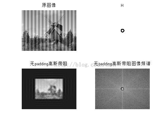
a.无padding过程:
显示原图像:
f=imread(windmill_noise.png');
figure,subplot(2,2,1),imshow(f);
title(‘原图像');
F=fft2(f);
[M N]=size(f);
f=double(f);
fc=fftshift(F);
s=log(1+abs(fc));
subplot(2,2,2),imshow(s,[]);
title(‘原图像频谱');<span style="color:#cc66cc;">
理想带阻滤波器滤波效果:
[u1,v1]=dftuv(M,N);
d1=sqrt(u1.^2+v1.^2);
w=5;
 D0=15;
ba= d1<(D0-w/2) | d1>(D0+w/2);
H=double(ba);
g=real(ifft2(H.*fft2(f)));
subplot(2,2,3),imshow(g,[]);
title(‘理想带阻');
F=fft2(g);
fc=fftshift(F);
s=log(1+abs(fc));
subplot(2,2,4),imshow(s,[]);
title(理想带阻频谱');
巴特沃斯带阻滤波:
n=3;
H = 1./(1 + (w*d1./(d1.^2-D0^2)).^(2*n));
g=real(ifft2(H.*fft2(f)));
figure,subplot(2,2,1),imshow(g,[]);
 title(‘btr');
F=fft2(g);
fc=fftshift(F);
s=log(1+abs(fc));
subplot(2,2,2),imshow(s,[]);
 title(‘btr频谱图');
高斯带阻滤波:
H = 1-exp(-1/2*(((d1.^2)-D0^2)./(d1*w)).^2);
g=real(ifft2(H.*fft2(f)));
subplot(2,2,3),imshow(g,[]);
title(‘高斯带阻');
F=fft2(g);
fc=fftshift(F);
s=log(1+abs(fc));
subplot(2,2,4),imshow(s,[]);
title(‘高斯带阻频谱');
(2)主要MATLAB源码:
① dftfilt.m
function g=dftfilt(f,H)
F=fft2(f,size(H,1),size(H,2));
g=real(ifft2(H.*F));
g=g(1:size(f,1),1:size(f,2));
② dftuv.m
function [u,v]=dftuv(m,n)
u=0:(m-1);
v=0:(n-1);
idx=find(u>m/2);
u(idx)=u(idx)-m;
idy=find(v>n/2);
v(idy)=v(idy)-n;
[v,u]=meshgrid(v,u);
③ pad1.m
%本文件包含paddedsize.m和dftuv.m及dftfilt.m三个文件
f=imread('D:\test\windmill_noise.png');
 figure,subplot(2,2,1),imshow(f); title('原图像');
F=fft2(f);
[M N]=size(f);
f=double(f);
%fc=ifft2(fft2(f));
fc=fftshift(F);
s=log(1+abs(fc));
% subplot(2,2,2),imshow(s,[]);  title('原图像频谱');                  %原图像频谱
%##########################
PQ=paddedsize(size(f));
[u,v]=dftuv(PQ(1),PQ(2));
[u1,v1]=dftuv(M,N); %没有padding
d1=sqrt(u1.^2+v1.^2);

 w=10;%带宽                              理想带阻滤波
 D0=15;

ba= d1<(D0-w/2) | d1>(D0+w/2);
H=double(ba);
subplot(2,2,2),imshow(fftshift(H),[]);  title('H');
%H = 1-exp(-1/2*(((d1.^2)-D0^2)./(d1*w)).^2);%高斯带阻滤波器
% H=fftshift(H);
% H=ifftshift(H);
% h=(-1).^(u1+v1);
% hh=ifft2(h);
H=real(ifft2(H));
% subplot(2,2,2),imshow(H,[]);  title('H');
H1=imag(ifft2(H)); H=H+1i*H1;
H=ifftshift(H);
% H=H.*hh;
H=fft2(H,900,1200);
% subplot(2,2,2),imshow(ifft(real(H)),[]);  title('H');
F=fft2(f,900,1200);

%  F=fftshift(F);
% H=H(1:size(f,1),1:size(f,2));
% F=F(1:size(f,1),1:size(f,2));
tmp=H.*F;
g=real(ifft2(H.*F));
%subplot(2,2,3),imshow(ifftshift(log(1+abs(F.*H))),[]); title('无padding高斯带阻图像频谱');
%g=g(226:675,301:900);
% g=g(1:size(f,1),1:size(f,2));
subplot(2,2,3),imshow(g,[]); title('无padding高斯带阻');
F=fft2(g);
fc=fftshift(F);
s=log(1+abs(fc));
  subplot(2,2,4),imshow(s,[]); title('无padding高斯带阻图像频谱');
④ pad2.m
%本文件包含paddedsize.m和dftuv.m及dftfilt.m三个文件
f=imread('D:\test\windmill_noise.png');
figure,subplot(2,2,1),imshow(f); title('原图像');
F=fft2(f);
[M N]=size(f);
f=double(f);
fc=fftshift(F);
s=log(1+abs(fc));
subplot(2,2,2),imshow(s,[]); title('原图像频谱'); %原图像频谱
%##########################
% PQ=paddedsize(size(f));
% [u,v]=dftuv(PQ(1),PQ(2));
[u1,v1]=dftuv(M,N); %没有padding
d1=sqrt(u1.^2+v1.^2);
%d0=0.05*PQ(2);
%d0=0.1*N;
d0=15;
% F=fft2(f,PQ(1),PQ(2));
% H=1-(1-exp(-(u1.^2+v1.^2)/(2*(d0^2)))); %高斯高通滤波
% %g=dftfilt(f,H);
% g=real(ifft2(H.*fft2(f)));
% subplot(2,2,3),imshow(g,[]); title('高斯high通滤波');
% F=fft2(g);
% fc=fftshift(F);
% s=log(1+abs(fc));
% subplot(2,2,4),imshow(s,[]); title('高斯滤波后的图像频谱'); %高斯滤波后的图像频谱
% %###########################
% d=sqrt(u.^2+v.^2);
% H=1-1./(1+(d1/d0).^2); %巴特沃兹高通滤波
% %g=dftfilt(f,H);
% g=real(ifft2(H.*fft2(f)));
% figure,subplot(2,2,1),imshow(g,[]); title('巴特沃兹high通滤波');
% F=fft2(g);
% fc=fftshift(F);
% s=log(1+abs(fc));
% subplot(2,2,2),imshow(s,[]); title('巴特沃兹high通滤波后的图像频谱'); %巴特沃兹低通滤波后的图像频谱
% %##########################
% h=double(d1<=d0); %理想高通滤波
% %g=dftfilt(f,H);
% g=real(ifft2(H.*fft2(f)));
% H=1-double(d1<=d0);
% subplot(2,2,3),imshow(g,[]); title('理想high通滤波');
% F=fft2(g);
% fc=fftshift(F);
% s=log(1+abs(fc));
% subplot(2,2,4),imshow(s,[]); title('理想high通滤波后的图像频谱'); %理想低通滤波后的图像频谱
%#####################
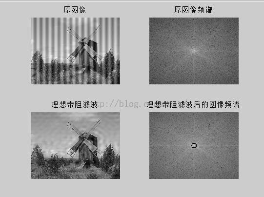
w=5;%带宽 理想带阻滤波
% % D0=sqrt(209*209+298*298);
D0=15;
ba= d1<(D0-w/2) | d1>(D0+w/2);
H=double(ba);
%g=dftfilt(f,H);
g=real(ifft2(H.*fft2(f)));
subplot(2,2,3),imshow(g,[]); title('理想带阻滤波');
F=fft2(g);
fc=fftshift(F);
s=log(1+abs(fc));
subplot(2,2,4),imshow(s,[]); title('理想带阻滤波后的图像频谱'); %理想带阻滤波后的图像频谱
%###########################
n=3; %3阶巴特沃斯滤波器
H = 1./(1 + (w*d1./(d1.^2-D0^2)).^(2*n));
%g=dftfilt(f,H);
g=real(ifft2(H.*fft2(f)));
figure,subplot(2,2,1),imshow(g,[]); title('巴特沃斯带阻滤波');
F=fft2(g);
fc=fftshift(F);
s=log(1+abs(fc));
subplot(2,2,2),imshow(s,[]); title('巴特沃斯带阻滤波图像频谱'); %巴特沃斯带阻滤波后的图像频谱
%#########################
H = 1-exp(-1/2*(((d1.^2)-D0^2)./(d1*w)).^2);%高斯带阻滤波器
%g=dftfilt(f,H);
g=real(ifft2(H.*fft2(f)));
subplot(2,2,3),imshow(g,[]); title('高斯带阻滤波器');
F=fft2(g);
fc=fftshift(F);
s=log(1+abs(fc));
subplot(2,2,4),imshow(s,[]); title('高斯带阻滤波后的图像频谱'); %高斯带阻滤波后的图像频谱
% %###########################
% v0=15;
% u0=0;
% d1=((u-M/2-u0).^2 + (v-N/2-v0).^2).^(1/2);
% d2=((u-M/2-u0).^2 + (v-N/2+v0).^2).^(1/2);
% H=double(d0<d1 & d0<d2);%理想陷波带阻滤波器
% g=dftfilt(f,H);
% subplot(2,2,3),imshow(g,[]);
% F=fft2(g);
% fc=fftshift(F);
% s=log(1+abs(fc));
% subplot(2,2,4),imshow(s,[]); %理想陷波带阻滤波后的图像频谱
% %H=1/(1+(D0^2/(d1.*d2)).^2); ⑤ pad3.m
%本文件包含paddedsize.m和dftuv.m及dftfilt.m三个文件
f=imread('D:\test\windmill_noise.png');
figure,subplot(2,2,1),imshow(f); title('原图像');
F=fft2(f);
[M N]=size(f);
f=double(f);
fc=fftshift(F);
s=log(1+abs(fc));
subplot(2,2,2),imshow(s,[]); title('原图像频谱'); %原图像频谱
%##########################
[u1,v1]=dftuv(M,N); %没有padding
d1=sqrt(u1.^2+v1.^2);
d0=15;
%#####################
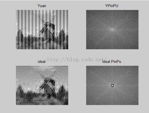
w=5;%带宽 理想带阻滤波
D0=15;
ba= d1<(D0-w/2) | d1>(D0+w/2);
H=double(ba);
g=real(ifft2(H.*fft2(f)));
subplot(2,2,3),imshow(g,[]); title('理想带阻滤波');
F=fft2(g);
fc=fftshift(F);
s=log(1+abs(fc));
subplot(2,2,4),imshow(s,[]); title('理想带阻滤波后的图像频谱'); %理想带阻滤波后的图像频谱
%###########################
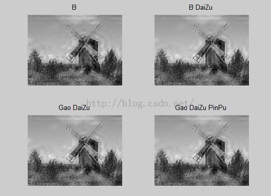
n=3; %3阶巴特沃斯滤波器
H = 1./(1 + (w*d1./(d1.^2-D0^2)).^(2*n));
g=real(ifft2(H.*fft2(f)));
figure,subplot(2,2,1),imshow(g,[]); title('巴特沃斯带阻滤波');
F=fft2(g);
fc=fftshift(F);
s=log(1+abs(fc));
subplot(2,2,2),imshow(s,[]); title('巴特沃斯带阻滤波图像频谱'); %巴特沃斯带阻滤波后的图像频谱
%#########################
H = 1-exp(-1/2*(((d1.^2)-D0^2)./(d1*w)).^2);%高斯带阻滤波器
g=real(ifft2(H.*fft2(f)));
subplot(2,2,3),imshow(g,[]); title('高斯带阻滤波器');
F=fft2(g);
fc=fftshift(F);
s=log(1+abs(fc));
subplot(2,2,4),imshow(s,[]); title('高斯带阻滤波后的图像频谱'); %高斯带阻滤波后的图像频谱 ⑥ paddedsize.m
function PQ = paddedsize(AB, CD, PARAM)
%PADDEDSIZE Computes padded sizes useful for FFT-based filtering.
%   PQ = PADDEDSIZE(AB), where AB is a two-element size vector,
%   computes the two-element size vector PQ = 2*AB.
%
%   PQ = PADDEDSIZE(AB, 'PWR2') computes the vector PQ such that
%   PQ(1) = PQ(2) = 2^nextpow2(2*m), where m is MAX(AB).
%
%   PQ = PADDEDSIZE(AB, CD), where AB and CD are two-element size
%   vectors, computes the two-element size vector PQ.  The elements
%   of PQ are the smallest even integers greater than or equal to
%   AB + CD - 1.
%
%   PQ = PADDEDSIZE(AB, CD, 'PWR2') computes the vector PQ such that
%   PQ(1) = PQ(2) = 2^nextpow2(2*m), where m is MAX([AB CD]).

%   Copyright 2002-2004 R. C. Gonzalez, R. E. Woods, & S. L. Eddins
%   Digital Image Processing Using MATLAB, Prentice-Hall, 2004
%   $Revision: 1.5 $  $Date: 2003/08/25 14:28:22 $

if nargin == 1
   PQ  = 2*AB;
elseif nargin == 2 & ~ischar(CD)
   PQ = AB + CD - 1;
   PQ = 2 * ceil(PQ / 2);
elseif nargin == 2
   m = max(AB); % Maximum dimension.

   % Find power-of-2 at least twice m.
   P = 2^nextpow2(2*m);
   PQ = [P, P];
elseif nargin == 3
   m = max([AB CD]); % Maximum dimension.
   P = 2^nextpow2(2*m);
   PQ = [P, P];
else
   error('Wrong number of inputs.')
end
以上代码的处理结果:
4.附录:
function R = imnoise2(type, M, N, a, b)
%IMNOISE2 Generates an array of random numbers with specified PDF.
%   R = IMNOISE2(TYPE, M, N, A, B) generates an array, R, of size
%   M-by-N, whose elements are random numbers of the specified TYPE
%   with parameters A and B. If only TYPE is included in the
%   input argument list, a  single random number of the specified
%   TYPE and default parameters shown below is generated. If only
%   TYPE, M, and N are provided, the default parameters shown below
%   are used.  If M = N = 1, IMNOISE2 generates a single random
%   number of the specified TYPE and parameters A and B.
%
%   Valid values for TYPE and parameters A and B are:
%
%   'uniform'       Uniform random numbers in the interval (A, B).
%                   The default values are (0, 1).
%   'gaussian'      Gaussian random numbers with mean A and standard
%                   deviation B. The default values are A = 0, B = 1.
%   'salt & pepper' Salt and pepper numbers of amplitude 0 with
%                   probability Pa = A, and amplitude 1 with
%                   probability Pb = B. The default values are Pa =
%                   Pb = A = B = 0.05.  Note that the noise has
%                   values 0 (with probability Pa = A) and 1 (with
%                   probability Pb = B), so scaling is necessary if
%                   values other than 0 and 1 are required. The noise
%                   matrix R is assigned three values. If R(x, y) =
%                   0, the noise at (x, y) is pepper (black).  If
%                   R(x, y) = 1, the noise at (x, y) is salt
%                   (white). If R(x, y) = 0.5, there is no noise
%                   assigned to coordinates (x, y).
%   'lognormal'     Lognormal numbers with offset A and shape
%                   parameter B. The defaults are A = 1 and B =
%                   0.25.
%   'rayleigh'      Rayleigh noise with parameters A and B. The
%                   default values are A = 0 and B = 1.
%   'exponential'   Exponential random numbers with parameter A.  The
%                   default is A = 1.
%   'erlang'        Erlang (gamma) random numbers with parameters A
%                   and B.  B must be a positive integer. The
%                   defaults are A = 2 and B = 5.  Erlang random
%                   numbers are approximated as the sum of B
%                   exponential random numbers.

%   Copyright 2002-2004 R. C. Gonzalez, R. E. Woods, & S. L. Eddins
%   Digital Image Processing Using MATLAB, Prentice-Hall, 2004
%   $Revision: 1.5 $  $Date: 2003/10/12 23:37:29 $

% Set default values.
if nargin == 1
   a = 0; b = 1;
   M = 1; N = 1;
elseif nargin == 3
   a = 0; b = 1;
end

% Begin processing. Use lower(type) to protect against input being
% capitalized.
switch lower(type)
case 'uniform'
   R = a + (b - a)*rand(M, N);
case 'gaussian'
   R = a + b*randn(M, N);
case 'salt & pepper'
   if nargin <= 3
      a = 0.05; b = 0.05;
   end
   % Check to make sure that Pa + Pb is not > 1.
   if (a + b) > 1
      error('The sum Pa + Pb must not exceed 1.')
   end
   R(1:M, 1:N) = 0.5;
   % Generate an M-by-N array of uniformly-distributed random numbers
   % in the range (0, 1). Then, Pa*(M*N) of them will have values <=
   % a. The coordinates of these points we call 0 (pepper
   % noise). Similarly, Pb*(M*N) points will have values in the range
   % > a & <= (a + b).  These we call 1 (salt noise).
   X = rand(M, N);
   c = find(X <= a);
   R(c) = 0;
   u = a + b;
   c = find(X > a & X <= u);
   R(c) = 1;
case 'lognormal'
   if nargin <= 3
      a = 1; b = 0.25;
   end
   R = a*exp(b*randn(M, N));
case 'rayleigh'
   R = a + (-b*log(1 - rand(M, N))).^0.5;
case 'exponential'
   if nargin <= 3
      a = 1;
   end
   if a <= 0
      error('Parameter a must be positive for exponential type.')
   end
   k = -1/a;
   R = k*log(1 - rand(M, N));
case 'erlang'
   if nargin <= 3
      a = 2; b = 5;
   end
   if (b ~= round(b) | b <= 0)
      error('Param b must be a positive integer for Erlang.')
   end
   k = -1/a;
   R = zeros(M, N);
   for j = 1:b
      R = R + k*log(1 - rand(M, N));
   end
otherwise
   error('Unknown distribution type.')
end<span style="color:#3333ff;">
</span>
② 生成周期噪声:
imnoise3.m
function [r, R, S] = imnoise3(M, N, C, A, B)
%IMNOISE3 Generates periodic noise.
%    [r, R, S] = IMNOISE3(M, N, C, A, B), generates a spatial
%    sinusoidal noise pattern, r, of size M-by-N, its Fourier
%    transform, R, and spectrum, S.  The remaining parameters are:
%
%    C is a K-by-2 matrix with K pairs of freq. domain coordinates (u,
%    v) that define the locations of impulses in the freq. domain. The
%    locations are with respect to the frequency rectangle center at
%    (floor(M/2) + 1, floor(N/2) + 1).  The impulse locations are spe-
%    cified as increments with respect to the center. For ex, if M =
%    N = 512, then the center is at (257, 257). To specify an impulse
%    at (280, 300) we specify the pair (23, 43); i.e., 257 + 23 = 280,
%    and 257 + 43 = 300. Only one pair of coordinates is required for
%    each impulse.  The conjugate pairs are generated automatically.
%
%    A is a 1-by-K vector that contains the amplitude of each of the
%    K impulse pairs. If A is not included in the argument, the
%    default used is A = ONES(1, K).  B is then automatically set to
%    its default values (see next paragraph).  The value specified
%    for A(j) is associated with the coordinates in C(j, 1:2).
%
%    B is a K-by-2 matrix containing the Bx and By phase components
%    for each impulse pair.  The default values for B are B(1:K, 1:2)
%    = 0.

%   Copyright 2002-2004 R. C. Gonzalez, R. E. Woods, & S. L. Eddins
%   Digital Image Processing Using MATLAB, Prentice-Hall, 2004
%   $Revision: 1.5 $  $Date: 2004/11/04 22:32:42 $

% Process input parameters.
[K, n] = size(C);
if nargin == 3
   A(1:K) = 1.0;
   B(1:K, 1:2) = 0;
elseif nargin == 4
   B(1:K, 1:2) = 0;
end

% Generate R.
R = zeros(M, N);
for j = 1:K
   u1 = M/2 + 1 + C(j, 1); v1 = N/2 + 1 + C(j, 2);
   R(u1, v1) = i * (A(j)/2) * exp(i*2*pi*C(j, 1) * B(j, 1)/M);
   % Complex conjugate.
   u2 = M/2 + 1 - C(j, 1); v2 = N/2 + 1 - C(j, 2);
   R(u2, v2) = -i * (A(j)/2) * exp(i*2*pi*C(j, 2) * B(j, 2)/N);
end

% Compute spectrum and spatial sinusoidal pattern.
S = abs(R);
r = real(ifft2(ifftshift(R)));
③ 低通滤波: lpfilter.m
function H = lpfilter(type, M, N, D0, n)
%LPFILTER Computes frequency domain lowpass filters.
%   H = LPFILTER(TYPE, M, N, D0, n) creates the transfer function of
%   a lowpass filter, H, of the specified TYPE and size (M-by-N). To
%   view the filter as an image or mesh plot, it should be centered
%   using H = fftshift(H).
%
%   Valid values for TYPE, D0, and n are:
%
%   'ideal'    Ideal lowpass filter with cutoff frequency D0. n need
%              not be supplied.  D0 must be positive.
%
%   'btw'      Butterworth lowpass filter of order n, and cutoff
%              D0.  The default value for n is 1.0.  D0 must be
%              positive.
%
%   'gaussian' Gaussian lowpass filter with cutoff (standard
%              deviation) D0.  n need not be supplied.  D0 must be
%              positive.

%   Copyright 2002-2004 R. C. Gonzalez, R. E. Woods, & S. L. Eddins
%   Digital Image Processing Using MATLAB, Prentice-Hall, 2004
%   $Revision: 1.8 $  $Date: 2004/11/04 22:33:16 $

% Use function dftuv to set up the meshgrid arrays needed for
% computing the required distances.
[U, V] = dftuv(M, N);

% Compute the distances D(U, V).
D = sqrt(U.^2 + V.^2);

% Begin filter computations.
switch type
case 'ideal'
   H = double(D <= D0);
case 'btw'
   if nargin == 4
      n = 1;
   end
   H = 1./(1 + (D./D0).^(2*n));
case 'gaussian'
   H = exp(-(D.^2)./(2*(D0^2)));
otherwise
   error('Unknown filter type.')
end
④ 带通滤波:bpfilter.m
function H=bpfilter(type, M, N, D0,n,W)
if nargin == 4
   n = 1; % Default value of n.
end

% Generate highpass filter.
Hlp = bsfilter(type, M, N, D0, n,W);
H = 1 - Hlp;
⑤ 带阻滤波:bsfilter.m
function H=bsfilter(type, M, N, D0,n,W)
[U, V] = dftuv(M, N);

% Compute the distances D(U, V).
D = sqrt(U.^2 + V.^2);

% Begin filter computations.
switch type
case 'ideal'
   if D < (D0-W/2)|D > (D0+W/2)
       H=1;
   else
       H=0;
   end
case 'btw'
   if nargin == 4
      n = 1;
   end
   H = 1./(1 + (D./(D.^2-D0^2)).^(2*n));
case 'gaussian'
   H = 1-exp-1/2*(((D.^2)-D0^2)./(D*W)).^2;
otherwise
   error('Unknown filter type.')
end
⑥ 高通滤波:hpfilter.m
function H = hpfilter(type, M, N, D0, n)
%HPFILTER Computes frequency domain highpass filters.
%   H = HPFILTER(TYPE, M, N, D0, n) creates the transfer function of
%   a highpass filter, H, of the specified TYPE and size (M-by-N).
%   Valid values for TYPE, D0, and n are:
%
%   'ideal'    Ideal highpass filter with cutoff frequency D0.  n
%              need not be supplied. D0 must be positive.
%
%   'btw'      Butterworth highpass filter of order n, and cutoff
%              D0.  The default value for n is 1.0. D0 must be
%              positive.
%
%   'gaussian' Gaussian highpass filter with cutoff (standard
%              deviation) D0. n need not be supplied. D0 must be
%              positive.

%   Copyright 2002-2004 R. C. Gonzalez, R. E. Woods, & S. L. Eddins
%   Digital Image Processing Using MATLAB, Prentice-Hall, 2004
%   $Revision: 1.4 $  $Date: 2003/08/25 14:28:22 $

% The transfer function Hhp of a highpass filter is 1 - Hlp,
% where Hlp is the transfer function of the corresponding lowpass
% filter.  Thus, we can use function lpfilter to generate highpass
% filters.

if nargin == 4
   n = 1; % Default value of n.
end

% Generate highpass filter.
Hlp = lpfilter(type, M, N, D0, n);
H = 1 - Hlp;
⑦ adpmedian.m
function f=adpmedian(g,smax)
if(smax<=1)||(smax/2==round(smax/2))||(smax~=round(smax))
    error('smax must be an odd inger>1')
end
[M,N]=size(g);
f=g;
f(:)=0;
alreadyprocessed=false(size(g));
for k=3:2:smax
    zmin=ordfilt2(g,1,ones(k,k),'symmetric');
    zmax=ordfilt2(g,k*k,ones(k,k),'symmetric');
    zmed=medfilt2(g,[k,k],'symmetric');
    processusinglevelB=(zmed>zmin)&(zmax>zmed)&~alreadyprocessed;
    zB=(g>zmin)&(zmax>g);
    outputzxy=processusinglevelB &zB;
    outputzmed=processusinglevelB &~zB;
    f(outputzxy)=g(outputzxy);
    f(outputzmed)=g(outputzmed);
    alreadyprocessed=alreadyprocessed|processusinglevelB;
    if all( alreadyprocessed(:))
        break;
    end
end
⑧ 改变图像的存储类:changeclass.m
function image = changeclass(class, varargin)
%CHANGECLASS changes the storage class of an image.
%  I2 = CHANGECLASS(CLASS, I);
%  RGB2 = CHANGECLASS(CLASS, RGB);
%  BW2 = CHANGECLASS(CLASS, BW);
%  X2 = CHANGECLASS(CLASS, X, 'indexed');

%  Copyright 1993-2002 The MathWorks, Inc.  Used with permission.
%  $Revision: 1.2 $  $Date: 2003/02/19 22:09:58 $

switch class
case 'uint8'
   image = im2uint8(varargin{:});
case 'uint16'
   image = im2uint16(varargin{:});
case 'double'
   image = im2double(varargin{:});
otherwise
   error('Unsupported IPT data class.');
end
⑨ 空间域滤波: spfilt.m
function f = spfilt(g, type, m, n, parameter)
%SPFILT Performs linear and nonlinear spatial filtering.
%   F = SPFILT(G, TYPE, M, N, PARAMETER) performs spatial filtering
%   of image G using a TYPE filter of size M-by-N. Valid calls to
%   SPFILT are as follows:
%
%     F = SPFILT(G, 'amean', M, N)       Arithmetic mean filtering.
%     F = SPFILT(G, 'gmean', M, N)       Geometric mean filtering.
%     F = SPFILT(G, 'hmean', M, N)       Harmonic mean filtering.
%     F = SPFILT(G, 'chmean', M, N, Q)   Contraharmonic mean
%                                        filtering of order Q. The
%                                        default is Q = 1.5.
%     F = SPFILT(G, 'median', M, N)      Median filtering.
%     F = SPFILT(G, 'max', M, N)         Max filtering.
%     F = SPFILT(G, 'min', M, N)         Min filtering.
%     F = SPFILT(G, 'midpoint', M, N)    Midpoint filtering.
%     F = SPFILT(G, 'atrimmed', M, N, D) Alpha-trimmed mean filtering.
%                                        Parameter D must be a
%                                        nonnegative even integer;
%                                        its default value is D = 2.
%
%   The default values when only G and TYPE are input are M = N = 3,
%   Q = 1.5, and D = 2.

%   Copyright 2002-2004 R. C. Gonzalez, R. E. Woods, & S. L. Eddins
%   Digital Image Processing Using MATLAB, Prentice-Hall, 2004
%   $Revision: 1.6 $  $Date: 2003/10/27 20:07:00 $

% Process inputs.
if nargin == 2
   m = 3; n = 3; Q = 1.5; d = 2;
elseif nargin == 5
   Q = parameter; d = parameter;
elseif nargin == 4
   Q = 1.5; d = 2;
else
   error('Wrong number of inputs.');
end

% Do the filtering.
switch type
case 'amean'
   w = fspecial('average', [m n]);
   f = imfilter(g, w, 'replicate');
case 'gmean'
   f = gmean(g, m, n);
case 'hmean'
   f = harmean(g, m, n);
case 'chmean'
   f = charmean(g, m, n, Q);
case 'median'
   f = medfilt2(g, [m n], 'symmetric');
case 'max'
   f = ordfilt2(g, m*n, ones(m, n), 'symmetric');
case 'min'
   f = ordfilt2(g, 1, ones(m, n), 'symmetric');
case 'midpoint'
   f1 = ordfilt2(g, 1, ones(m, n), 'symmetric');
   f2 = ordfilt2(g, m*n, ones(m, n), 'symmetric');
   f = imlincomb(0.5, f1, 0.5, f2);
case 'atrimmed'
   if (d <= 0) | (d/2 ~= round(d/2))
      error('d must be a positive, even integer.')
   end
   f = alphatrim(g, m, n, d);
otherwise
   error('Unknown filter type.')
end

%-------------------------------------------------------------------%
function f = gmean(g, m, n)
%  Implements a geometric mean filter.
inclass = class(g);
g = im2double(g);
% Disable log(0) warning.
warning off;
f = exp(imfilter(log(g), ones(m, n), 'replicate')).^(1 / m / n);
warning on;
f = changeclass(inclass, f);

%-------------------------------------------------------------------%
function f = harmean(g, m, n)
%  Implements a harmonic mean filter.
inclass = class(g);
g = im2double(g);
f = m * n ./ imfilter(1./(g + eps),ones(m, n), 'replicate');
f = changeclass(inclass, f);

%-------------------------------------------------------------------%
function f = charmean(g, m, n, q)
%  Implements a contraharmonic mean filter.
inclass = class(g);
g = im2double(g);
f = imfilter(g.^(q+1), ones(m, n), 'replicate');
f = f ./ (imfilter(g.^q, ones(m, n), 'replicate') + eps);
f = changeclass(inclass, f);

%-------------------------------------------------------------------%
function f = alphatrim(g, m, n, d)
%  Implements an alpha-trimmed mean filter.
inclass = class(g);
g = im2double(g);
f = imfilter(g, ones(m, n), 'symmetric');
for k = 1:d/2
   f = imsubtract(f, ordfilt2(g, k, ones(m, n), 'symmetric'));
end
for k = (m*n - (d/2) + 1):m*n
   f = imsubtract(f, ordfilt2(g, k, ones(m, n), 'symmetric'));
end
f = f / (m*n - d);
f = changeclass(inclass, f);
⑩ 入口函数:paddedsize.m
function PQ=paddedsize(AB,CD,PARAM)
if nargin==1
      PQ=2*AB;
  elseif nargin==2&~ischar(CD)
      PQ=AB+CD-1;
      PQ=2*ceil(PQ/2);
  elseif nargin==2
      m=max(AB);
      P=2^nextpow2(2*m);
      PQ=[P,P];
  elseif nargin==3
      m=max([AB,CD]);
      P=2^nextpow2(2*m);
      PQ=[P,P];
  else
      error('wrong number of inputs.')
  end
%%%%%%%%%%%%%%%%%%%%%%%%%%%%%%%%%%
function [u,v]=dftuv(m,n)
u=0:(m-1);
v=0:(n-1);
idx=find(u>m/2);
u(idx)=u(idx)-m;
idy=find(v>n/2);
v(idy)=v(idy)-n;
[v,u]=meshgrid(v,u);
%%%%%%%%%%%%%%%%%%%%%%%%%%%%%%%%%%%
function g=dftfilt(f,H)
F=fft2(f,size(H,1),size(H,2));
g=real(ifft2(H.*F));
g=g(1:size(f,1),1:size(f,2));
%%%%%%%%%%%%%%%%%%%%%%%%%%%%%%%%%%%
%本文件包含paddedsize.m和dftuv.m及dftfilt.m三个文件
f=imread('D:\test\windmill_noise.png');
figure,subplot(2,2,1),imshow(f);
F=fft2(f);
fc=fftshift(F);
s=log(1+abs(fc));
subplot(2,2,2),imshow(s,[]);                    %原图像频谱
PQ=paddedsize(size(f));
[u,v]=dftuv(PQ(1),PQ(2));
d0=0.05*PQ(2);
F=fft2(f,PQ(1),PQ(2));
H=exp(-(u.^2+v.^2)/(2*(d0^2)));       %高斯低通滤波
g=dftfilt(f,H);
subplot(2,2,3),imshow(g,[]);
F=fft2(g);
fc=fftshift(F);
s=log(1+abs(fc));
subplot(2,2,4),imshow(s,[]);       %高斯滤波后的图像频谱
d=sqrt(u.^2+v.^2);
H=1./(1+(d/d0).^2);                  %巴特沃兹低通滤波
g=dftfilt(f,H);
figure,subplot(2,2,1),imshow(g,[]);
F=fft2(g);
fc=fftshift(F);
s=log(1+abs(fc));
subplot(2,2,2),imshow(s,[]);      %巴特沃兹低通滤波后的图像频谱
h=double(d<=d0);                    %理想低通滤波
g=dftfilt(f,H);
H=double(d<=d0);
subplot(2,2,3),imshow(g,[]);
F=fft2(g);
fc=fftshift(F);
s=log(1+abs(fc));
subplot(2,2,4),imshow(s,[]);         %理想低通滤波后的图像频谱