Geometric Scaling
http://homepages.inf.ed.ac.uk/rbf/HIPR2/scale.htm
Geometric Scaling
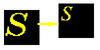
Common Names: Scale, Zoom, Shrink, Pixel Replication, Pixel Interpolation, Subsampling
Brief Description
The scale operator performs a geometric transformation which can be used to shrink or zoom the size of an image (or part of an image). Image reduction, commonly known as ![]() subsampling, is performed by replacement (of a group ofpixel values by one arbitrarily chosen pixel value from within this group) or by interpolating between pixel values in a local neighborhoods. Image zooming is achieved by pixel replication or by interpolation. Scaling is used to change the visual appearance of an image, to alter the quantity of information stored in a scene representation, or as a low-level preprocessor in multi-stage image processing chain which operates on features of a particular scale. Scaling is a special case of affine transformation.
subsampling, is performed by replacement (of a group ofpixel values by one arbitrarily chosen pixel value from within this group) or by interpolating between pixel values in a local neighborhoods. Image zooming is achieved by pixel replication or by interpolation. Scaling is used to change the visual appearance of an image, to alter the quantity of information stored in a scene representation, or as a low-level preprocessor in multi-stage image processing chain which operates on features of a particular scale. Scaling is a special case of affine transformation.
![]()
How It Works
Scaling compresses or expands an image along the coordinate directions. As different techniques can be used to subsample and zoom, each is discussed in turn.
Figure 1 illustrates the two methods of sub-sampling. In the first, one pixel value within a local neighborhood is chosen (perhaps randomly) to be representative of its surroundings. (This method is computationally simple, but can lead to poor results if the sampling neighborhoods are too large.) The second method interpolates between pixel values within a neighborhood by taking a statistical sample (such as the mean) of the local intensity values.
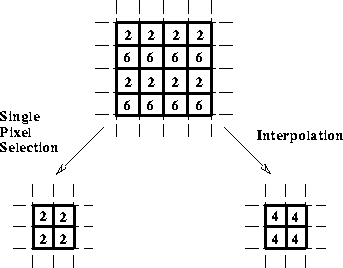
Figure 1 Methods of subsampling. a) Replacement with upper left pixel. b) Interpolation using the mean value.
An image (or regions of an image) can be zoomed either through pixel replication or interpolation. Figure 2 shows how pixel replication simply replaces each original image pixel by a group of pixels with the same value (where the group size is determined by the scaling factor). Alternatively, interpolation of the values of neighboring pixels in the original image can be performed in order to replace each pixel with an expanded group of pixels. Most implementations offer the option of increasing the actual dimensions of the original image, or retaining them and simply zooming a portion of the image within the old image boundaries.
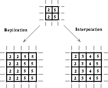
Figure 2 Methods of zooming. a) Replication of a single pixel value. b) Interpolation.
![]()
Guidelines for Use
Image sampling is a fundamental operation of any image processing system. In a digital computer, images are represented as arrays of finite size numbers. The size of the image array is determined by the number of sampling pointsmeasured. The information at each sampling position in the array represents the average irradiance over the small sampling area and is quantized into a finite number of bits.
How many sampling points and quantization levels are required to make a good approximation to the continuous image? The ![]() resolution of the image increases as we increase the number of sampling and quantization levels. However, large values for these parameters also increase the image storage space and processing requirements. Therefore, the decision of how to set these parameters must involve striking a compromise between these competing objectives. Fortunately,
resolution of the image increases as we increase the number of sampling and quantization levels. However, large values for these parameters also increase the image storage space and processing requirements. Therefore, the decision of how to set these parameters must involve striking a compromise between these competing objectives. Fortunately, ![]() sampling theory gives us some boundaries within which to make an otherwise largely qualitative decision. If we model images as bandlimited signals, Fourier analysis tells us that sampling at frequencies greater than twice the image bandwidths allows us to recover images without error (by lowpass filtering the sampled image). However if the sampling frequencies are below this
sampling theory gives us some boundaries within which to make an otherwise largely qualitative decision. If we model images as bandlimited signals, Fourier analysis tells us that sampling at frequencies greater than twice the image bandwidths allows us to recover images without error (by lowpass filtering the sampled image). However if the sampling frequencies are below this ![]() Nyquist limit, then the spectrum will be distorted and information will be lost. This phenomenon is known as
Nyquist limit, then the spectrum will be distorted and information will be lost. This phenomenon is known as ![]() aliasing.
aliasing.
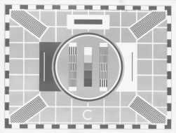
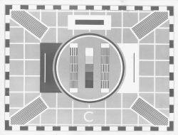
We can witness this effect by subsampling the test image
The effect of reducing the sampling grid size by a half is shown in
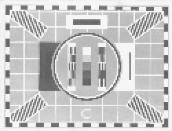
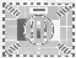
The maximum number of intensity levels, or quantization levels, is held constant in this example. Also, since the display area used in each example is the same, pixels in the lower resolution images are duplicated in order to fill out the display field. Reducing the resolution by a factor of 4, 8, and 16 are shown in
and
respectively.
Next we consider the different methods of implementing subsampling using a series of examples based on the basic image
This image is first subsampled using (i) pixel replacement, as shown in
and (ii) pixel interpolation, as shown in
(In each case the image is reduced by a factor of 4.) Notice how the latter produces a smoother image with less loss of information on the upper watch face.
We can zoom in on a region of the watch image using both (i) pixel replication
and (ii) interpolation
Again the interpolation method produced a slightly smoother result, but the differences in quality are rather insignificant as the neighborhood size used was small (i.e. 2) to keep the computation time down when processing such a large image. (Note, the zooming facilities used here produced different sized outputs; i.e. pixel replication created an image which was increased in size by the scale factor and pixel interpolation cropped the zoomed image to remain within the boundaries of the original image. To aid viewing, the pixel replicated image was manually cropped to cut it down to the approximate size of the interpolated image.)
Zooming another, smaller image
shows more clearly the effects of increasing the neighborhood size. Using a scaling factor of 3, pixel replication produces
and pixel interpolation yields
At this scale factor, we begin to see the undesirable effects of block edge features appearing in the replicated image.
Scaling algorithms are implemented on hardware (e.g. a zooming facility is provided on most frame grabbers) as well as software. Subsampling has utility in applications where information can be reduced without losing the main characteristics of the image, while image expansion is often used to examine details and local image information.
Interactive Experimentation
You can interactively experiment with this operator by clicking here.
Exercises
- Using the binary images


and

make a collage by scaling each image so that the object in the second image can fit within the object in the first image, and the third within the second.
- Explore the effects of subsampling noisy images. Using the image

-- which has been contaminated with salt and pepper noise and

-- which has been corrupted by Gaussian noise. Subsample each image using both the pixel replacement and pixel interpolation methods. Does one algorithm cope with noise better than the other? Which type of noise is more corrupting to the subsampled image.
- Using objects of different sizes, determine the scale of subsampling at which the objects are no longer visible in the output images. Experiment with images

and

Repeat this analysis for both types of subsampling.
References
E. Davies Machine Vision: Theory, Algorithms and Practicalities, Academic Press, 1990, pp 465 - 469, 470.
R. Gonzalez and P. Wintz Digital Image Processing, 2nd edition, Addison-Wesley Publishing Company, 1987, pp 22 - 26.
A. Jain Fundamentals of Digital Image Processing, Prentice-Hall, 1986, Chap. 4.
A. Marion An Introduction to Image Processing, Chapman and Hall, 1991, Chap. 5.
D. Vernon Machine Vision, Prentice-Hall, 1991
