【SPP-net】《Spatial Pyramid Pooling in Deep Convolutional Networks for Visual Recognition》

ECCV-2014

---

目录

---

1 Motivation

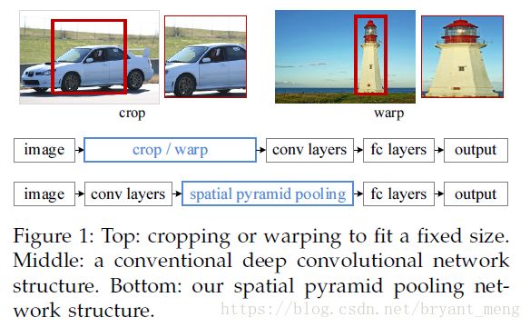
• Existing deep convolutional neural networks (CNNs) require a fixed-size (e.g., 224×224) input image. This requirement is “artificial” and may reduce the recognition accuracy for the images or sub-images of an arbitrary size/scale.

limits both the aspect ratio and the scale of the input image

• When applied to images of arbitrary sizes, current methods mostly fit the input image to the fixed size, either via cropping or via warping, as shown in Figure 1 (top).

In this work, we equip the networks with a more principled pooling strategy, “spatial pyramid pooling”, to eliminate the above requirement.

主要改进（与RCNN比）

• 共享卷积计算
• 空间金字塔池化

2 Advantages

• Our method computes convolutional features 30-170× faster than the recent and most accurate method R-CNN (and 24-64× faster overall) while achieving better or comparable accuracy on Pascal VOC 2007.（快）
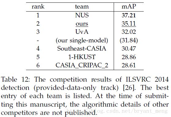
• In ImageNet Large Scale Visual Recognition Challenge (ILSVRC) 2014, our methods rank #2 in object detection and #3 in image classification among all 38 teams. （准）

3 Method（Deep Networks with spatial pyramid pooling）

SPP-net（fig1 bottom）

We add an SPP layer on top of the last convolutional layer.The SPP layer pools the features and generates fixed length outputs, which are then fed into the fully connected layers (or other classifiers). In other words, we perform some information “aggregation” at a deeper stage of the network hierarchy (between convolutional layers and fully-connected layers) to avoid the need for cropping or warping at the beginning.

3.1 Convolutional Layers and Feature Maps

• 55-th filter：circle shape
• 66-th filter：^ shape
• 118-th filter：v shape

So why do CNNs require a fixed input size?

The deep network described above needs a fixed image size. However, we notice that the requirement of fixed sizes is only due to the fully-connected layers that demand fixed-length vectors as inputs.

3.2 The Spatial Pyramid Pooling Layer

全部用的是max pooling
k*M dimention

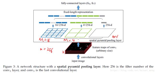
maxpooling 后的效果如下

max pooling 的计算方法如下
Consider the feature maps after conv5 that have a size of a×a (e.g., 13×13). With a pyramid level of n×n bins

话不多说，for examples，下图，把 conv5 的13*13*256 分别 max pooling 到 3*3*256、 2*2*256、1*1*256，filter 的 size 和step 用以下的公式， ⌊ ⌋ ⌊   ⌋ 表示 floor， ⌈ ⌉ ⌈   ⌉ 表示 ceil

• 3*3*256：size = ⌈133⌉=5 ⌈ 13 3 ⌉ = 5 , stride = ⌊133⌋=4 ⌊ 13 3 ⌋ = 4 ，然后 ⌊13−54⌋+1=3 ⌊ 13 − 5 4 ⌋ + 1 = 3
• 2*2*256：size = ⌈132⌉=7 ⌈ 13 2 ⌉ = 7 , stride = ⌊132⌋=6 ⌊ 13 2 ⌋ = 6 ，然后 ⌊13−76⌋+1=2 ⌊ 13 − 7 6 ⌋ + 1 = 2
• 1*1*256：size = ⌈131⌉=13 ⌈ 13 1 ⌉ = 13 , stride = ⌊131⌋=13 ⌊ 13 1 ⌋ = 13 ，然后 ⌊13−1313⌋+1=1 ⌊ 13 − 13 13 ⌋ + 1 = 1
  

3.3 Training the Network with the Spatial Pyramid Pooling Layer

3.3.1 Single-size training

As in previous works, we first consider a network taking a fixed-size input (224×224) cropped from images.
conv5 13*13

3.3.2 Multi-size training

Rather than crop a smaller 180*180 region, we resize the aforementioned 224*224 region to 180*180. So the regions
at both scales differ only in resolution but not in content/layout.

• 224*224 conv5 13*13
• 180*180 conv5 10*10

In theory, we could use more scales/aspect ratios, with one network for each scale/aspect ratio and all networks sharing weights, or we could develop a varying-size implementation to avoid network switching. We will study this in the future.（更多尺寸will study in the future）

Note that the above single/multi-size solutions are for training only. At the testing stage, it is straightforward to apply SPP-net on images of any sizes.（测试可以是任何的size）

下面是训练和测试的流程图

4 SPP-net for image classification

4.1 Experiments on ImageNet 2012 Classification

4.1.1 Baseline Network Architectures

table2 （a）

• ZF-5
• Convnet*-5（AlexNet中，We put the two pooling layers after conv2 and conv3 (instead of after conv1 and conv2））
• Overfeat5
• Overfeat7

4.1.2 Multi-level Pooling Improves Accuracy

table2 （b）

• The training and testing sizes are both 224*224.
• use a 4-level pyramid. The pyramid is （6*6, 3*3, 2*2, 1*1） (totally 50 bins).
• still use the standard 10-view prediction with each view a 224*224 crop

（b）比（a）好 not simply due to more parameters; rather, it is because the multi-level pooling is robust to the variance in object deformations and spatial layout.

作者 做了另外一个实验
To show this, we train another ZF-5 network with a different 4-level pyramid: （4*4, 3*3, 2*2, 1*1）(totally 30 bins). This network has fewer parameters than its no-SPP counterpart, because its fc6 layer has 30*256-d inputs instead of 36*256-d. The top-1/top-5 errors of this network are 35.06/14.04. This result is similar to the 50-bin pyramid above (34.98/14.14), but considerably better than the no-SPP counterpart (35.99/14.76).

4.1.3 Multi-size Training Improves Accuracy

table2 （c）

• The training and testing sizes are both 224*224.
• still use the standard 10-view prediction with each view a 224*224 crop

To the best of our knowledge, our method is the first one that trains a single network with input images of multiple scales/sizes.

4.1.4 Full-image Representations Improve Accuracy

table3

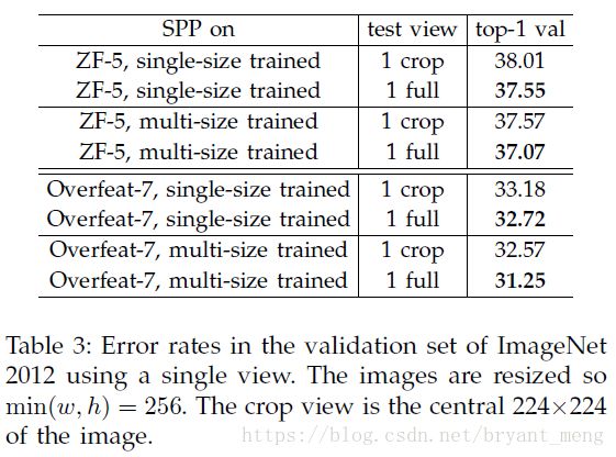
Comparing Table 2 and Table 3, we find that the combination of multiple views is substantially better than the single full-image view. However, the fullimage representations are still of good merits.

4.1.5 Multi-view Testing on Feature Maps

figrue 5（table4 最后一行） vs 10-view prediction（table4 倒数第二行）

we resize an image so min(w; h) = s，s 属于 （224; 256; 300; 360; 448; 560）

We use 18 views for each scale: one at the center, four at the corners, and four on the middle of each side, with/without flipping (when s = 224 there are 6 different views).

6 + 18*5 = 96

The combination of these 96 views reduces the top-5 error from 10.95% to 9.36%. Combining the two full image
views (with flipping) further reduces the top-5 error to 9.14%.

4.1.6 Summary and Results for ILSVRC 2014

table 4

6 + 18*5 = 96

The combination of these 96 views reduces the top-5 error from 10.95% to 9.36%. Combining the two full image
views (with flipping) further reduces the top-5 error to 9.14%.

结果排名 (table5)
After combining eleven models, our team’s result (8.06%) is ranked #3 among all 38 teams attending ILSVRC 2014.

we expect that it will further improve the advanced (deeper and larger) convolutional architectures in the future.

4.2 Experiments on VOC 2007 Classification

table 6

与别的方法对比下
table 8

4.3 Experiments on Caltech101

table7

与别的方法对比下

table 8

The fully-connected layers are less accurate, and the SPP layers are better. This is possibly because the object categories in Caltech101 are less related to those in ImageNet, and the deeper layers are more category-specialized.

5 SPP-net for object detection

5.1 Detection Algorithm

• ss 产生2000 candidate window
• resize min（w,h）= s
• extract the feature maps from the entire image（convnet）
• 4-level spatial pyramid (1*1, 2*2, 3*3, 6*6, totally 50 bins),This generates a 12,800-d (256*50) representation for each window
• fc
• Then we train a binary linear SVM classifier for each category on these features,ground truth 为 positive window，iou <0.3 negetive， 与 negetive overlap 超过70%的 直接pass
• iou [0.5,1] 为正，[0.1,0.5) 负，each mini-batch 25% positive，bbox regression to predict window as RCNN, 用 conv5的特征，the windows used for the regression training are overlapping with ground truth window by at least 50%

5.2 Detection Results

5.3 Complexity and Running Time

table 9

5.4 Model Combination for Detection

5.5 ILSVRC 2014 Detection

6 存在的问题

最后，通过上面的性能评价可以看到，SPP-Net在速度上有大幅的提升，其所提出的共享卷积计算的思想在后续的Fast R-CNN与Faster R-CNN中都在沿用，但是从SPP-Net的训练过程可以看出，它是无法finetune卷积层的，这个问题在Fast RCNN中通过多任务损失函数与Roi Pooling提出得以解决。

SPP-Net的训练过程依然是一个多阶段的训练，这一点和R-CNN一样，并为改进。 由于是多阶段训练，过程中需要存储大量特征。

---

补充知识

1Bag-of-Words

1.1 起源

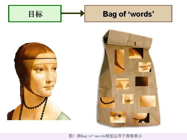
Bag of words模型最初被用在文本分类中，将文档表示成特征矢量。它的基本思想是假定对于一个文本，忽略其词序和语法、句法，仅仅将其看做是一些词汇的集合，而文本中的每个词汇都是独立的。简单说就是讲每篇文档都看成一个袋子（因为里面装的都是词汇，所以称为词袋，Bag of words 即因此而来），然后看这个袋子里装的都是些什么词汇，将其分类。如果文档中猪、马、牛、羊、山谷、土地、拖拉机这样的词汇多些，而银行、大厦、汽车、公园这样的词汇少些，我们就倾向于判断它是一篇描绘乡村的文档，而不是描述城镇的。举个例子，有如下两个文档：

• 文档一：Bob likes to play basketball, Jim likes too.

• 文档二：Bob also likes to play football games.

基于这两个文本文档，构造一个词典：

• Dictionary = {1:”Bob”, 2. “like”, 3. “to”, 4. “play”, 5. “basketball”, 6. “also”, 7. “football”，8. “games”, 9. “Jim”, 10. “too”}。

这个词典一共包含10个不同的单词，利用词典的索引号，上面两个文档每一个都可以用一个10维向量表示（用整数数字0~n（n为正整数）表示某个单词在文档中出现的次数）：

• 1：[1, 2, 1, 1, 1, 0, 0, 0, 1, 1]

• 2：[1, 1, 1, 1 ,0, 1, 1, 1, 0, 0]

向量中每个元素表示词典中相关元素在文档中出现的次数(下文中，将用单词的直方图表示)。不过，在构造文档向量的过程中可以看到，我们并没有表达单词在原来句子中出现的次序（这是 Bag-of-words 模型的缺点之一，不过瑕不掩瑜甚至在此处无关紧要）。

1.2 为什么要用BoW模型描述图像？

SIFT 特征虽然也能描述一幅图像，但是每个 SIFT 矢量都是 128 维的，而且一幅图像通常都包含成百上千个 SIFT 矢量，在进行相似度计算时，这个计算量是非常大的，通行的做法是用聚类算法对这些矢量数据进行聚类，然后用聚类中的一个簇代表 BOW 中的一个视觉词，将同一幅图像的 SIFT 矢量映射到视觉词序列生成码本，这样每一幅图像只用一个码本矢量来描述，这样计算相似度时效率就大大提高了。

1.3 构建BOW码本步骤

• 假设训练集有M 幅图像，对训练图象集进行预处理。包括图像增强，分割，图像统一格式，统一规格等等。

• 提取SIFT特征。对每一幅图像提取SIFT特征（每一幅图像提取多少个SIFT特征不定）。每一个SIFT特征用一个128维的描述子矢量表示，假设 M 幅图像共提取出 N 个SIFT特征。

• 用 K-means对 2 中提取的N个 SIFT 特征进行聚类，聚类中心有k个（在BOW模型中聚类中心我们称它们为视觉词），码本的长度也就为k，计算每一幅图像的每一个SIFT特征到这k个视觉词的距离，并将其映射到距离最近的视觉词中（即将该视觉词的对应词频+1）。

完成这一步后，每一幅图像就变成了一个与视觉词序列相对应的词频矢量。

设视觉词序列为{眼睛 鼻子 嘴}（k=3），则训练集中的图像变为：

第一幅图像：[1 0 0]

第二幅图像：[5 3 4]……

• 构造码本。码本矢量归一化因为每一幅图像的SIFT特征个数不定，所以需要归一化。如上述例子，归一化后为[1 0 0],1/12*[5 3 4].测试图像也需经过预处理，提取SIFT特征，将这些特征映射到为码本矢量，码本矢量归一化，最后计算其与训练码本的距离，对应最近距离的训练图像认为与测试图像匹配。

当然，在提取sift特征的时候，可以将图像打成很多小的patch，然后对每个patch提取SIFT特征。

总结一下，整个过程其实就做了三件事，首先提取对 n 幅图像分别提取SIFT特征，然后对提取的整个SIFT特征进行k-means聚类得到 k 个聚类中心作为视觉单词表，最后对每幅图像以单词表为规范对该幅图像的每一个SIFT特征点计算它与单词表中每个单词的距离，最近的+1，便可得到该幅图像的码本。实际上第三步是一个统计的过程，所以BOW中向量元素都是非负的。Yunchao Gong 2012年NIPS上有一篇用二进制编码用于图像快速检索的文章就是针对这类元素是非负的特征而设计的编码方案。

用 K-meas 把 sift 特征聚类，聚类中心构成视觉单词表

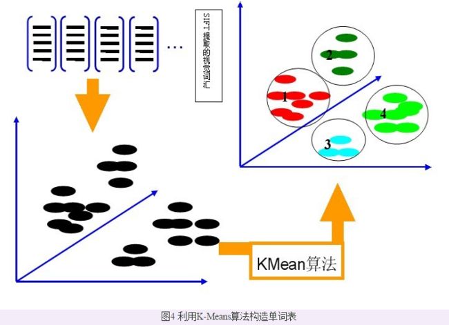
计算每个sift 特征到视觉单词表 中每个单词的距离，最近的+1，便可得到该幅图像的码本

---

参考
【1】目标识别：Bag-of-words表示图像
【2】Object Detection系列（二） SPP-Net