机器学习课程梳理 (01) ——线性回归
来源:http://openclassroom.stanford.edu/MainFolder/DocumentPage.php?course=DeepLearning&doc=exercises/ex2/ex2.html
在这个例子中,因为数据方差比较小,迭代500次可以得到非常近似的解。但是如同文中所讲,运行1500次可以得到更加精确的解,4位有效数字情况下和理论解相同。
Linear regression
Now, we will implement linear regression for this problem. Recall that the linear regression model is

and the batch gradient descent update rule is

1. Implement gradient descent using a learning rate of ![]() . Since Matlab/Octave and Octave index vectors starting from 1 rather than 0, you'll probably use theta(1) and theta(2) in Matlab/Octave to represent
. Since Matlab/Octave and Octave index vectors starting from 1 rather than 0, you'll probably use theta(1) and theta(2) in Matlab/Octave to represent ![]() and
and ![]() . Initialize the parameters to
. Initialize the parameters to ![]() (i.e.,
(i.e., ![]() ), and run one iteration of gradient descent from this initial starting point. Record the value of of
), and run one iteration of gradient descent from this initial starting point. Record the value of of ![]() and
and ![]() that you get after this first iteration. (To verify that your implementation is correct, later we'll ask you to check your values of
that you get after this first iteration. (To verify that your implementation is correct, later we'll ask you to check your values of ![]() and
and ![]() against ours.)
against ours.)
2. Continue running gradient descent for more iterations until ![]() converges. (this will take a total of about 1500 iterations). After convergence, record the final values of
converges. (this will take a total of about 1500 iterations). After convergence, record the final values of ![]() and
and ![]() that you get.
that you get.
Understanding ![]()
We'd like to understand better what gradient descent has done, and visualize the relationship between the parameters![]() and
and ![]() . In this problem, we'll plot
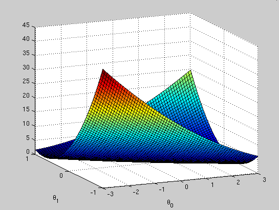
. In this problem, we'll plot ![]() as a 3D surface plot. (When applying learning algorithms, we don't usually try to plot
as a 3D surface plot. (When applying learning algorithms, we don't usually try to plot ![]() since usually
since usually ![]() is very high-dimensional so that we don't have any simple way to plot or visualize
is very high-dimensional so that we don't have any simple way to plot or visualize ![]() . But because the example here uses a very low dimensional
. But because the example here uses a very low dimensional ![]() , we'll plot
, we'll plot ![]() to gain more intuition about linear regression.) Recall that the formula for
to gain more intuition about linear regression.) Recall that the formula for ![]() is
is

What is the relationship between this 3D surface and the value of ![]() and
and ![]() that your implementation of gradient descent had found?
that your implementation of gradient descent had found?
Linear Regression
1. After your first iteration of gradient descent, verify that you get

If your answer does not exactly match this solution, you may have implemented something wrong. Did you get the correct![]() , but the wrong answer for
, but the wrong answer for ![]() ? (You might have gotten
? (You might have gotten ![]() ). If this happened, you probably updated the
). If this happened, you probably updated the ![]() terms sequentially, that is, you first updated
terms sequentially, that is, you first updated ![]() , plugged that value back into
, plugged that value back into ![]() , and then updated
, and then updated ![]() . Remember that you should not be basing your calculations on any intermediate values of
. Remember that you should not be basing your calculations on any intermediate values of ![]() that you would get this way.
that you would get this way.
2. After running gradient descent until convergence, verify that your parameters are approximately equal to the exact closed-form solution (which you will learn about in the next assignment):
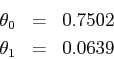
If you run gradient descent in MATLAB for 1500 iterations at a learning rate of 0.07, you should see these exact numbers for theta. If used fewer iterations, your answer should not differ by more than 0.01, or you probably did not iterate enough. For example, running gradient descent in MATLAB for 500 iterations gives theta = [0.7318, 0.0672]. This is close to convergence, but theta can still get closer to the exact value if you run gradient descent some more.
If your answer differs drastically from the solutions above, there may be a bug in your implementation. Check that you used the correct learning rate of 0.07 and that you defined the gradient descent update correctly. Then, check that your x and y vectors are indeed what you expect them to be. Remember that x needs an extra column of ones.
3. The predicted height for age 3.5 is 0.9737 meters, and for age 7 is 1.1975 meters.
Plot A plot of the training data with the best fit from gradient descent should look like the following graph.

Understanding ![]()
In your surface plot, you should see that the cost function ![]() approaches a minimum near the values of
approaches a minimum near the values of ![]() and
and ![]() that you found through gradient descent. In general, the cost function for a linear regression problem will be bowl-shaped with a global minimum and no local optima.
that you found through gradient descent. In general, the cost function for a linear regression problem will be bowl-shaped with a global minimum and no local optima.
The result is a plot like the following.

Now the location of the minimum is more obvious.