一起深入读懂Mahony互补滤波器
一起深入读懂Mahony互补滤波器
本文是Jesse Chen的原创文章,如有引用,请注明出处。本文
- 补全了论文Complementary Filter Design on the Special Orthogonal Group SO(3) 的绝大部分推导过程。
- 修正了论文的两处公式印刷错误。
- 通过求解微分方程,补充了滤波器收敛性数值仿真。
- 给出了direct complementary filter和passive complementary filter的对比数值仿真更多的仿真结果。
建议有兴趣的读者可以从网上下载论文 Complementary Filter Design on the Special Orthogonal Group SO(3) 对照本博文阅读。如果读者对本文的推导过程和仿真有需要讨论的地方,请邮件联系[email protected]
文章目录
- 一起深入读懂Mahony互补滤波器
- Filter Design and Error Criteria for Estimation on SO(3)
- Known Mathematical Identities
- Cost Function for the complementary filters
- Non-linear Complementary Filter Design on SO(3)
- A. Theoretical development of complementary filter on SO(3)
- B. Implementing a complementary filter on SO(3)
- Direct complementary filter
- Passive complementary filter
- C. Passive complementary filter design
- D. Simulation Results
- Attitude Extraction and Gyros Bias Estimation from Passive Complementary Filter
- A Quaternion-Based derivation of the passive complementary filter
- 回顾
- 参考文献
Filter Design and Error Criteria for Estimation on SO(3)
三种坐标系:
- A \mathcal{A} A表示惯性(固定)参考坐标系;
- B \mathcal{B} B表示固定在设备(body fixed frame)上的参考坐标系;
- E \mathcal{E} E表示估计参考坐标系;
定义固定在设备上的参考坐标系相对于惯性参考坐标系的姿态为 R = B A R R = {}_\mathcal{B}^\mathcal{A}R R=BAR,固定在设备上的参考坐标的角速度为 Ω = B Ω \Omega = {}^\mathcal{B}\Omega Ω=BΩ。
姿态系统的动力学方程为:
R ˙ = R Ω × \dot{R} = R\Omega_\times R˙=RΩ×
其中 Ω × \Omega_\times Ω×表示skew-symmetric矩阵, Ω × a = Ω × a \Omega_\times\mathbf{a} = \Omega\times\mathbf{a} Ω×a=Ω×a。从skew-symmetric matrix得到对应向量的函数为:
Ω = vex ( Ω × ) \Omega = \operatorname{vex}\left(\Omega_\times\right) Ω=vex(Ω×)
做VSLAM的同学都知道姿态系统的动力学方程可以写成如下的四元数形式:
q ˙ = 1 2 q ⊗ p ( Ω ) \dot{q} = \frac{1}{2}q\otimes\mathbf{p}\left(\Omega\right) q˙=21q⊗p(Ω)
其中 q q q表示一个单位四元数 q = { ( s , v ) ∣ s 2 + ∣ v ∣ 2 = 1 } q = \left\{\left(s,\mathbf{v}\right)\,\vert\,s^2 + \left\vert\mathbf{v}\right\vert^2 = 1\right\} q={(s,v)∣s2+∣v∣2=1}, p ( Ω ) \mathbf{p}\left(\Omega\right) p(Ω)表示和向量 Ω \Omega Ω对应的纯四元数 p ( Ω ) = ( 0 , Ω ) ′ \mathbf{p}\left(\Omega\right) = \left(0,\,\Omega\right)^\prime p(Ω)=(0,Ω)′。
陀螺仪测量到的角速度 Ω y \Omega_y Ωy是基于固定在设备上的参考坐标系的,
Ω y = Ω + b ( t ) + μ Ω \Omega_y = \Omega + b\left(t\right) + \mu_\Omega Ωy=Ω+b(t)+μΩ
其中 Ω \Omega Ω是角速度的真实值, b ( t ) b\left(t\right) b(t)是缓慢变化的偏差(bias), μ Ω \mu_\Omega μΩ表示噪声。陀螺仪的bias破坏了陀螺仪测量值( Ω y \Omega_y Ωy)中的低频信息,但是 Ω y \Omega_y Ωy的高频信息还是很不错的。
加速度计和磁力计的测量值会一起提供姿态旋转 R y R_y Ry的代数估计。互补滤波器的目标是融合低频测量 R y R_y Ry和高频变换量测量 Ω y \Omega_y Ωy来获得姿态的一个好的估计 R ^ \hat{R} R^。
R ^ \hat{R} R^可以看成对固定在设备上的参考坐标系的旋转矩阵 R R R的一个估计。旋转 R ^ \hat{R} R^自身也可以看成是估计参考坐标系的旋转:
R ^ = E A R ^ : E → A \hat{R} = {}_\mathcal{E}^\mathcal{A}\hat{R}\,:\,\mathcal{E}\to\mathcal{A} R^=EAR^:E→A
估计误差也是一个旋转:
R ~ = R ^ T R : B → A \widetilde{R} = \hat{R}^T R\,:\,\mathcal{B}\to\mathcal{A} R =R^TR:B→A
互补滤波器的设计目标是找到对于 R ^ ( t ) ∈ S O ( 3 ) \hat{R}\left(t\right)\in SO\left(3\right) R^(t)∈SO(3)的一个动力学系统使得 R ~ → I \widetilde{R}\to I R →I。
Jesse’s Comment:
- 对于较短的时间间隔 t t t,我们可以得到:
R ( t ) = R exp ( Ω × t ) R\left(t\right) = R\exp\left(\Omega_\times t\right) R(t)=Rexp(Ω×t)
上式两边对 t = 0 t=0 t=0求导,可以得到:
R ˙ = R d d t exp ( Ω × t ) ∣ t = 0 = R exp ( Ω × t ) ∣ t = 0 Ω × = R Ω × \dot{R} = R\frac{d}{dt}\exp\left(\Omega_\times t\right)\Big\vert_{t=0} = R\exp\left(\Omega_\times t\right)\Big\vert_{t=0}\Omega_\times = R\Omega_\times R˙=Rdtdexp(Ω×t)∣∣∣t=0=Rexp(Ω×t)∣∣∣t=0Ω×=RΩ× - R ∈ S O ( 3 ) R\in SO\left(3\right) R∈SO(3)且 R ^ ∈ S O ( 3 ) \hat{R}\in SO\left(3\right) R^∈SO(3),因此 R ~ ∈ S O ( 3 ) \widetilde{R}\in SO\left(3\right) R ∈SO(3);
- 如果 R ^ = R \hat{R} = R R^=R,那么 R ~ = R ^ T R = I \widetilde{R} = \hat{R}^T R = I R =R^TR=I;
Known Mathematical Identities
为了阅读本博文方便,这里列举出一些用到的数学公式:
π a ( R ~ ) = 1 2 ( R ~ − R ~ T ) , π s ( R ~ ) = 1 2 ( R ~ + R ~ T ) \pi_a\left(\widetilde{R}\right) = \frac{1}{2}\left(\widetilde{R} - \widetilde{R}^T\right),\qquad\pi_s\left(\widetilde{R}\right) = \frac{1}{2}\left(\widetilde{R} + \widetilde{R}^T\right) πa(R )=21(R −R T),πs(R )=21(R +R T)
显然 π a \pi_a πa和 π s \pi_s πs会分别得到skew-symmetic矩阵和symmetric矩阵。
R ~ = π a ( R ~ ) + π s ( R ~ ) , π a ( R ~ ) T = − π a ( R ~ ) , π s ( R ~ ) T = π s ( R ~ ) \widetilde{R} = \pi_a\left(\widetilde{R}\right) + \pi_s\left(\widetilde{R}\right),\ \pi_a\left(\widetilde{R}\right)^T = -\pi_a\left(\widetilde{R}\right),\ \pi_s\left(\widetilde{R}\right)^T = \pi_s\left(\widetilde{R}\right) R =πa(R )+πs(R ), πa(R )T=−πa(R ), πs(R )T=πs(R )
假设 ( θ , a ) \left(\theta, \mathbf{a}\right) (θ,a)是 R ~ \widetilde{R} R 的角-轴表示,那么
R ~ = exp ( θ a × ) , log ( R ~ ) = θ a × cos ( θ ) = 1 2 ( tr ( R ~ ) − 1 ) , a × = 1 sin ( θ ) π a ( R ~ ) \begin{aligned} \widetilde{R} &= \exp\left(\theta\mathbf{a}_\times\right),\qquad\log\left(\widetilde{R}\right) = \theta\mathbf{a}_\times \\ \cos\left(\theta\right) &= \frac{1}{2}\left(\operatorname{tr}\left(\widetilde{R}\right) - 1\right),\qquad\mathbf{a}_\times = \frac{1}{\sin\left(\theta\right)}\pi_a\left(\widetilde{R}\right) \end{aligned} R cos(θ)=exp(θa×),log(R )=θa×=21(tr(R )−1),a×=sin(θ)1πa(R )
Cost Function for the complementary filters
Mahony在论文中提出complementary filter的设计cost function为:
E t : = ∥ I 3 − R ~ ∥ 2 = 1 2 tr ( I 3 − R ~ ) = ( 1 − cos ( θ ) ) = 2 sin 2 ( θ 2 ) E_t := \left\| I_3 - \widetilde{R}\right\|^2 = \frac{1}{2}\operatorname{tr}\left(I_3 - \widetilde{R}\right) = \left(1 - \cos\left(\theta\right)\right) = 2\sin^2\left(\frac{\theta}{2}\right) Et:=∥∥∥I3−R ∥∥∥2=21tr(I3−R )=(1−cos(θ))=2sin2(2θ)
Non-linear Complementary Filter Design on SO(3)
A. Theoretical development of complementary filter on SO(3)
对于 R ∈ S O ( 3 ) R\in SO\left(3\right) R∈SO(3)和任意 a ∈ R 3 \mathbf{a}\in\mathbb{R}^3 a∈R3,都有:
( R a ) × = R a × R T \left(R\mathbf{a}\right)_\times = R\mathbf{a}_\times R^T (Ra)×=Ra×RT
所以,对于 R ˙ = R Ω × \dot{R} = R\Omega_\times R˙=RΩ×有:
R ˙ = R Ω × = ( R Ω ) × R \begin{aligned} \dot{R} &= R\Omega_\times = \left(R\Omega\right)_\times R \end{aligned} R˙=RΩ×=(RΩ)×R
Mahony提出如下的动力学系统:
R ^ ˙ = ( R Ω + R ^ ω ( R ^ , R ) ) × R ^ \dot{\hat{R}} = \left(R\Omega + \hat{R}\omega\left(\hat{R}, R\right)\right)_\times\hat{R} R^˙=(RΩ+R^ω(R^,R))×R^
其中 ω ( R ^ , R ) ∈ E \omega\left(\hat{R}, R\right)\in\mathcal{E} ω(R^,R)∈E是修正项,当 R ^ = R \hat{R} = R R^=R时, ω ( R ^ , R ) = 0 \omega\left(\hat{R}, R\right) = \mathbf{0} ω(R^,R)=0。
这就是direct complementary filter的动态方程。
对于 R ~ \widetilde{R} R ,其动力学方程为:
R ~ ˙ = R ^ T ( R Ω + R ^ ω ) × T R + R ^ T ( R Ω ) × R = R ^ T ( R ^ ω R ^ T ) T R = ω × T R ~ = − ω × R ~ \begin{aligned} \dot{\widetilde{R}} &= \hat{R}^T\left(R\Omega + \hat{R}\omega\right)_\times^T R + \hat{R}^T\left(R\Omega\right)_\times R = \hat{R}^T\left(\hat{R}\omega\hat{R}^T\right)^T R \\ &= \omega_\times^T\widetilde{R} = -\omega_\times\widetilde{R} \end{aligned} R ˙=R^T(RΩ+R^ω)×TR+R^T(RΩ)×R=R^T(R^ωR^T)TR=ω×TR =−ω×R
Jesse’s Comment: 推导上式的关键是:
R ~ = R ^ T R ⇒ R ~ ˙ = ( R ^ ˙ ) T R + R ^ T R ˙ \widetilde{R} = \hat{R}^T R\qquad\Rightarrow\qquad\dot{\widetilde{R}} = \left(\dot{\hat{R}}\right)^T R + \hat{R}^T\dot{R} R =R^TR⇒R ˙=(R^˙)TR+R^TR˙
分别将
R ^ ˙ = ( R Ω + R ^ ω ( R ^ , R ) ) × R ^ R ˙ = R Ω × = ( R Ω ) × R \begin{aligned} \dot{\hat{R}} &= \left(R\Omega + \hat{R}\omega\left(\hat{R}, R\right)\right)_\times\hat{R} \\ \dot{R} &= R\Omega_\times = \left(R\Omega\right)_\times R \end{aligned} R^˙R˙=(RΩ+R^ω(R^,R))×R^=RΩ×=(RΩ)×R
带入即可。
修正项 ω \omega ω可以选为:
ω = k e s t vex ( π a ( R ~ ) ) ⇔ ω × = k e s t π a ( R ~ ) , k e s t > 0 \omega = k_{est}\operatorname{vex}\left(\pi_a\left(\widetilde{R}\right)\right)\Leftrightarrow\omega_\times = k_{est}\pi_a\left(\widetilde{R}\right),\, k_{est} > 0 ω=kestvex(πa(R ))⇔ω×=kestπa(R ),kest>0
Lemma 3.1: 如果direct complementary filter的动态方程为:
R ^ ˙ = ( R Ω + R ^ ω ) × R ^ = ( ( R Ω ) × + k e s t R ^ π a ( R ~ ) R ^ T ) R ^ , with R ^ ( 0 ) = R ^ 0 \dot{\hat{R}} = \left(R\Omega + \hat{R}\omega\right)_\times\hat{R} = \left(\left(R\Omega\right)_\times + k_{est}\hat{R}\pi_a\left(\widetilde{R}\right)\hat{R}^T\right)\hat{R},\quad\text{with}\,\,\hat{R}\left(0\right) = \hat{R}_0 R^˙=(RΩ+R^ω)×R^=((RΩ)×+kestR^πa(R )R^T)R^,withR^(0)=R^0
那么
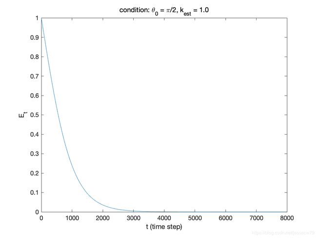
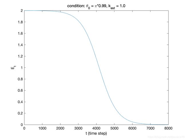
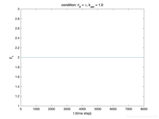
E ˙ t = − 2 k e s t cos 2 ( θ 2 ) E t \dot{E}_t = -2k_{est}\cos^2\left(\frac{\theta}{2}\right)E_t E˙t=−2kestcos2(2θ)Et
对于任何的初始条件 R ^ 0 \hat{R}_0 R^0,只要
θ 0 = 1 2 ∥ log ( R ~ 0 ) ∥ < π \theta_0 = \frac{1}{\sqrt{2}}\left\|\log\left(\widetilde{R}_0\right)\right\| < \pi θ0=21∥∥∥log(R 0)∥∥∥<π
那么 E t → 0 E_t\to 0 Et→0且 R ^ ( t ) → R ( t ) \hat{R}\left(t\right)\to R\left(t\right) R^(t)→R(t)。
Jesse’s Comment:
解微分方程:
E ˙ t = − 2 k e s t cos 2 ( θ 2 ) E t \dot{E}_t =-2k_{est}\cos^2\left(\frac{\theta}{2}\right)E_t E˙t=−2kestcos2(2θ)Et
初始值:
E 0 = 2 sin 2 ( θ 0 2 ) E_0 = 2\sin^2\left(\frac{\theta_0}{2}\right) E0=2sin2(2θ0)
可以得到:
E t = 2 sin 2 ( θ 0 2 ) e − k e s t ( cos θ + 1 ) t E_t = 2\sin^2\left(\frac{\theta_0}{2}\right)e^{-k_{est}\left(\cos\theta + 1\right)t} Et=2sin2(2θ0)e−kest(cosθ+1)t
其中 θ \theta θ是时变的,初始值 θ ( 0 ) = θ 0 \theta\left(0\right) = \theta_0 θ(0)=θ0。显然 cos θ + 1 ≥ 0 \cos\theta + 1 \geq 0 cosθ+1≥0,只要 θ 0 < π \theta_0 < \pi θ0<π, E t → 0 E_t\to 0 Et→0。
我们可以进行数值仿真,得到 θ 0 \theta_0 θ0取不同值时, E t E_t Et的曲线,
假设初始值 R ~ = R ~ 0 \widetilde{R} = \widetilde{R}_0 R =R 0,那么
log ( R ~ 0 ) = θ 0 a × \log\left(\widetilde{R}_0\right) = \theta_0\mathbf{a}_\times log(R 0)=θ0a×
对上式两边取Frobenius范数,且 ∣ a ∣ 2 = 1 2 ∥ a × ∥ 2 \left\vert\mathbf{a}\right\vert^2 = \frac{1}{2}\left\|\mathbf{a}_\times\right\|^2 ∣a∣2=21∥a×∥2, a \mathbf{a} a是单位向量( ∣ a ∣ = 1 \left\vert\mathbf{a}\right\vert = 1 ∣a∣=1),那么
∥ log ( R ~ 0 ) ∥ = θ 0 ∥ a × ∥ ⇒ θ 0 = 1 2 ∥ log ( R ~ 0 ) ∥ \begin{aligned} \left\|\log\left(\widetilde{R}_0\right)\right\| &= \theta_0\left\|\mathbf{a}_\times\right\| \\ \Rightarrow\qquad\qquad\theta_0 &= \frac{1}{\sqrt{2}}\left\|\log\left(\widetilde{R}_0\right)\right\| \end{aligned} ∥∥∥log(R 0)∥∥∥⇒θ0=θ0∥a×∥=21∥∥∥log(R 0)∥∥∥
B. Implementing a complementary filter on SO(3)
Direct complementary filter
如图所示,direct complementary filter采用测量的旋转 R y R_y Ry作为其中的一个输入。direct complementary filter存在的问题是:测量到的 R y R_y Ry通常可能会被高频噪声破坏掉。噪声会通过 ( R y Ω y ) \left(R_y\Omega_y\right) (RyΩy)传递到最终的输出。

Passive complementary filter
在passive complementary filter中, ( R y Ω y ) \left(R_y\Omega_y\right) (RyΩy)中的 R y R_y Ry被估计的 R ^ \hat{R} R^所替换。这样做的优点是,如果滤波器表现良好,那么 R ^ \hat{R} R^是比 R y R_y Ry对真实旋转的一个更好的估计值。

C. Passive complementary filter design
如果采用估计值 R ^ \hat{R} R^做为反馈量,可以得到在估计参考坐标系下的滤波器动力学方程:
R ^ ˙ = ( R ^ Ω + R ^ ω ) × R ^ = ( R ^ Ω × R ^ T + k e s t R ^ π a ( R ~ ) R ^ T ) R ^ = R ^ ( Ω × + k e s t π a ( R ~ ) ) = R ^ ( Ω + ω ) × \dot{\hat{R}} = \left(\hat{R}\Omega + \hat{R}\omega\right)_\times\hat{R} = \left(\hat{R}\Omega_\times\hat{R}^T + k_{est}\hat{R}\pi_a\left(\widetilde{R}\right)\hat{R}^T\right)\hat{R} = \hat{R}\left(\Omega_\times + k_{est}\pi_a\left(\widetilde{R}\right)\right) = \hat{R}\left(\Omega + \omega\right)_\times R^˙=(R^Ω+R^ω)×R^=(R^Ω×R^T+kestR^πa(R )R^T)R^=R^(Ω×+kestπa(R ))=R^(Ω+ω)×
Jesse’s Comment:Mahony论文在 ( R ^ Ω × R ^ T + k e s t R ^ π a ( R ~ ) R ^ T ) R ^ \left(\hat{R}\Omega_\times\hat{R}^T + k_{est}\hat{R}\pi_a\left(\widetilde{R}\right)\hat{R}^T\right)\hat{R} (R^Ω×R^T+kestR^πa(R )R^T)R^前多印了一个 R ^ \hat{R} R^,以本博文为准。
该公式的推导过程如下:
R ^ ˙ = ( R ^ Ω + R ^ ω ) × R ^ = ( ( R ^ Ω ) × + ( R ^ ω ) × ) R ^ = ( R ^ Ω × R ^ T + R ^ ω × R ^ T ) R ^ = ( R ^ Ω × R ^ T + R ^ k e s t π a ( R ~ ) R ^ T ) R ^ = R ^ ( Ω × + k e s t π a ( R ~ ) ) R ^ T R ^ = R ^ ( Ω + ω × ) \begin{aligned} \dot{\hat{R}} &= \left(\hat{R}\Omega + \hat{R}\omega\right)_\times\hat{R} = \left(\left(\hat{R}\Omega\right)_\times + \left(\hat{R}\omega\right)_\times\right)\hat{R} \\ &= \left(\hat{R}\Omega_\times\hat{R}^T + \hat{R}\omega_\times\hat{R}^T\right)\hat{R} = \left(\hat{R}\Omega_\times\hat{R}^T + \hat{R}k_{est}\pi_a\left(\widetilde{R}\right)\hat{R}^T\right)\hat{R} \\ &= \hat{R}\left(\Omega_\times + k_{est}\pi_a\left(\widetilde{R}\right)\right)\hat{R}^T\hat{R} = \hat{R}\left(\Omega + \omega_\times\right) \end{aligned} R^˙=(R^Ω+R^ω)×R^=((R^Ω)×+(R^ω)×)R^=(R^Ω×R^T+R^ω×R^T)R^=(R^Ω×R^T+R^kestπa(R )R^T)R^=R^(Ω×+kestπa(R ))R^TR^=R^(Ω+ω×)
在Mahony论文中,还多次用到了一个结论:
Ad R ~ π a ( R ~ ) = R ~ π a ( R ~ ) R ~ T = π a ( R ~ ) \operatorname{Ad}_{\widetilde{R}}\pi_a\left(\widetilde{R}\right) = \widetilde{R}\pi_a\left(\widetilde{R}\right)\widetilde{R}^T = \pi_a\left(\widetilde{R}\right) AdR πa(R )=R πa(R )R T=πa(R )
由 R ~ ∈ S O ( 3 ) \widetilde{R}\in SO\left(3\right) R ∈SO(3),可得 R ~ R ~ T = R ~ T R ~ \widetilde{R}\widetilde{R}^T = \widetilde{R}^T\widetilde{R} R R T=R TR ,进而易得 R ~ \widetilde{R} R 和 ( R ~ − R ~ T ) \left(\widetilde{R} - \widetilde{R}^T\right) (R −R T)是可交换的。
Ad R ~ π a ( R ~ ) = R ~ π a ( R ~ ) R ~ T = 1 2 R ~ ( R ~ − R ~ T ) R ~ T = 1 2 ( R ~ − R ~ T ) R ~ R ~ T = 1 2 ( R ~ − R ~ T ) = π a ( R ~ ) \begin{aligned} \operatorname{Ad}_{\widetilde{R}}\pi_a\left(\widetilde{R}\right) &= \widetilde{R}\pi_a\left(\widetilde{R}\right)\widetilde{R}^T = \frac{1}{2}\widetilde{R}\left(\widetilde{R} - \widetilde{R}^T\right)\widetilde{R}^T \\ &= \frac{1}{2}\left(\widetilde{R} - \widetilde{R}^T\right)\widetilde{R}\widetilde{R}^T = \frac{1}{2}\left(\widetilde{R} - \widetilde{R}^T\right) \\ &= \pi_a\left(\widetilde{R}\right) \end{aligned} AdR πa(R )=R πa(R )R T=21R (R −R T)R T=21(R −R T)R R T=21(R −R T)=πa(R )
Lemma 3.2: 如果passive complementary filter的动力学方程为
R ^ ˙ = ( R ^ Ω + R ^ ω ) × R ^ = ( R ^ Ω × R ^ T + k e s t R ^ π a ( R ~ ) R ^ T ) R ^ = R ^ ( Ω × + k e s t π a ( R ~ ) ) = R ^ ( Ω + ω ) × \dot{\hat{R}} = \left(\hat{R}\Omega + \hat{R}\omega\right)_\times\hat{R} = \left(\hat{R}\Omega_\times\hat{R}^T + k_{est}\hat{R}\pi_a\left(\widetilde{R}\right)\hat{R}^T\right)\hat{R} = \hat{R}\left(\Omega_\times + k_{est}\pi_a\left(\widetilde{R}\right)\right) = \hat{R}\left(\Omega + \omega\right)_\times R^˙=(R^Ω+R^ω)×R^=(R^Ω×R^T+kestR^πa(R )R^T)R^=R^(Ω×+kestπa(R ))=R^(Ω+ω)×
那么
E ˙ t = − 2 k e s t cos 2 ( θ 2 ) E t \dot{E}_t = -2k_{est}\cos^2\left(\frac{\theta}{2}\right)E_t E˙t=−2kestcos2(2θ)Et
对于任意的初始值 R ^ 0 \hat{R}_0 R^0,只要
θ 0 = 1 2 ∥ log ( R ~ 0 ) ∥ < π \theta_0 = \frac{1}{\sqrt{2}}\left\|\log\left(\widetilde{R}_0\right)\right\| < \pi θ0=21∥∥∥log(R 0)∥∥∥<π
那么 E t → 0 E_t\to 0 Et→0且 R ^ ( t ) → R ( t ) \hat{R}\left(t\right)\to R\left(t\right) R^(t)→R(t)。
Jesse’s Comment:对于Lema 3.2,这里将 R ~ ˙ \dot{\widetilde{R}} R ˙的推导过程补上。
R ~ ˙ = ( R ^ ˙ ) T R + R ^ T R ˙ = ( R ^ ( Ω + ω ) × ) T R + R ^ T ( R Ω ) × R = ( Ω + ω ) × T R ^ T R + R ^ T R Ω × = ( Ω + ω ) × T R ~ + R ~ Ω × = − ( Ω + ω ) × R ~ + R ~ Ω × \begin{aligned} \dot{\widetilde{R}} &= \left(\dot{\hat{R}}\right)^T R + \hat{R}^T\dot{R} = \left(\hat{R}\left(\Omega + \omega\right)_\times\right)^T R + \hat{R}^T\left(R\Omega\right)_\times R \\ &= \left(\Omega + \omega\right)_\times^T\hat{R}^T R + \hat{R}^T R\Omega_\times = \left(\Omega + \omega\right)_\times^T\widetilde{R} + \widetilde{R}\Omega_\times \\ &= -\left(\Omega + \omega\right)_\times\widetilde{R} + \widetilde{R}\Omega_\times \end{aligned} R ˙=(R^˙)TR+R^TR˙=(R^(Ω+ω)×)TR+R^T(RΩ)×R=(Ω+ω)×TR^TR+R^TRΩ×=(Ω+ω)×TR +R Ω×=−(Ω+ω)×R +R Ω×
D. Simulation Results
按照论文中给出的仿真条件:
- 旋转矩阵的初始值 R ( 0 ) = I 3 R\left(0\right) = I_3 R(0)=I3;
- 偏差(deviation) R ~ \widetilde{R} R 的初始值对应的欧拉角为 [ 0 π 2 0 ] \left[\begin{array}{ccc} 0 & \frac{\pi}{2} & 0 \end{array}\right] [02π0];
- 角速度为 Ω = 0.3 e 3 \Omega = 0.3\,\mathbf{e}_3 Ω=0.3e3;
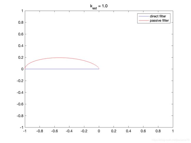
经过博文作者编程仿真,可以得到和Mahony论文一致的结果:
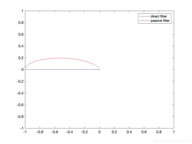
经过检查发现,论文中的仿真结果是在 k e s t = 1.0 k_{est} = 1.0 kest=1.0下获得的。让 k e s t k_{est} kest取不同的值,可以得到不同的仿真结果:
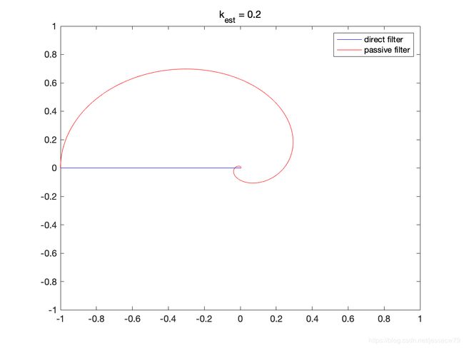

检查三个 k e s t k_{est} kest取值下,对应时刻direct filter和passive filter的仿真结果是否都在同心圆上,博文作者计算了不同的仿真时刻仿真结果相对圆心 ( 0 , 0 ) \left(0,0\right) (0,0)的半径差,取 k e s t = 0.2 k_{est} = 0.2 kest=0.2时候的结果来说明:

可以发现论文的结论是成立的,同一时刻direct complementary filter的仿真结果和passive complementary filter的仿真结果是在同心圆上的。(注意:半径差绝对值的量级是 1 0 − 14 10^{-14} 10−14)
Attitude Extraction and Gyros Bias Estimation from Passive Complementary Filter
在定理4.1的证明中需要用到一个结论:
b ~ T b ^ ˙ = 1 2 tr ( b ~ × T b ^ ˙ × ) \widetilde{\mathbf{b}}^T\dot{\hat{\mathbf{b}}} = \frac{1}{2}\operatorname{tr}\left(\widetilde{\mathbf{b}}_\times^T\dot{\hat{\mathbf{b}}}_\times\right) b Tb^˙=21tr(b ×Tb^˙×)
注意:论文原文中的结论不正确,以本博文给出的这个结论为准。
A Quaternion-Based derivation of the passive complementary filter
基于很多估计和控制算法是基于四元数,因此Mahony给出了基于四元数实现passive complementary filter的公式。
定义单位四元数误差 q ~ \widetilde{q} q :
q ~ = q ^ − 1 ⊗ q = [ s ~ v ~ ] \widetilde{q} = \hat{q}^{-1}\otimes q= \left[\begin{array}{c} \widetilde{s} \\ \widetilde{\mathbf{v}} \end{array}\right] q =q^−1⊗q=[s v ]
其中 q ~ \widetilde{q} q 和 R ~ \widetilde{R} R , q ^ \hat{q} q^和 R ^ \hat{R} R^, q q q和 R R R是对应的。
Thienel和Sanner在参考文献[2]中提出了
q ^ ˙ = 1 2 q ^ ⊗ p ( R ~ ( Ω y − b ^ + k e s t sgn ( s ~ ) v ~ ) ) \dot{\hat{q}} = \frac{1}{2}\hat{q}\otimes\mathbf{p}\left(\widetilde{R}\left(\Omega_y - \hat{\mathbf{b}} + k_{est}\operatorname{sgn}\left(\widetilde{s}\right)\widetilde{\mathbf{v}}\right)\right) q^˙=21q^⊗p(R (Ωy−b^+kestsgn(s )v ))
bias的估计 b ^ \hat{\mathbf{b}} b^的动态方程为:
b ^ ˙ = − k b sgn ( s ~ ) v ~ \dot{\hat{\mathbf{b}}} = -k_b\operatorname{sgn}\left(\widetilde{s}\right)\widetilde{\mathbf{v}} b^˙=−kbsgn(s )v
如果我们将 sgn ( s ~ ) \operatorname{sgn}\left(\widetilde{s}\right) sgn(s )替换成 2 s ~ 2\widetilde{s} 2s ,那么参考文献[2]中的滤波器等效于论文中提出的基于 S O ( 3 ) SO\left(3\right) SO(3)的direct complementary filter。
2 s ~ v ~ = 2 cos ( θ 2 ) sin ( θ 2 ) a = sin ( θ ) a = vex ( π a ( R ~ ) ) 2\widetilde{s}\widetilde{\mathbf{v}} = 2\cos\left(\frac{\theta}{2}\right)\sin\left(\frac{\theta}{2}\right)\mathbf{a} = \sin\left(\theta\right)\mathbf{a} = \operatorname{vex}\left(\pi_a\left(\widetilde{R}\right)\right) 2s v =2cos(2θ)sin(2θ)a=sin(θ)a=vex(πa(R ))
Jesse’s Comment: 对于单元四元数 q ~ \widetilde{q} q ,
q ~ = cos ( θ 2 ) + ( u x i + u y j + u z k ) sin ( θ 2 ) = cos ( θ 2 ) + a sin ( θ 2 ) \widetilde{q} = \cos\left(\frac{\theta}{2}\right) + \left(u_x\mathbf{i} + u_y\mathbf{j} + u_z\mathbf{k}\right)\sin\left(\frac{\theta}{2}\right) = \cos\left(\frac{\theta}{2}\right) + \mathbf{a}\sin\left(\frac{\theta}{2}\right) q =cos(2θ)+(uxi+uyj+uzk)sin(2θ)=cos(2θ)+asin(2θ)
所以,
s ~ = cos ( θ 2 ) v ~ = a sin ( θ 2 ) \widetilde{s} = \cos\left(\frac{\theta}{2}\right)\qquad\widetilde{\mathbf{v}} = \mathbf{a}\sin\left(\frac{\theta}{2}\right) s =cos(2θ)v =asin(2θ)
又由 π a ( R ~ ) = sin ( θ ) a × \pi_a\left(\widetilde{R}\right) = \sin\left(\theta\right)\mathbf{a}_\times πa(R )=sin(θ)a×,可知:
sin ( θ ) a = vex ( π a ( R ~ ) ) \sin\left(\theta\right)\mathbf{a} = \operatorname{vex}\left(\pi_a\left(\widetilde{R}\right)\right) sin(θ)a=vex(πa(R ))
因此
q ^ ˙ = 1 2 q ^ ⊗ p ( R ~ ( Ω y − b ^ + k e s t vex ( π a ( R ~ ) ) ) ) = 1 2 q ^ ⊗ p ( R ~ ( Ω y − b ^ ) + k e s t R ~ vex ( π a ( R ~ ) ) ) \dot{\hat{q}} = \frac{1}{2}\hat{q}\otimes\mathbf{p}\left(\widetilde{R}\left(\Omega_y - \hat{\mathbf{b}} + k_{est}\operatorname{vex}\left(\pi_a\left(\widetilde{R}\right)\right)\right)\right) = \frac{1}{2}\hat{q}\otimes\mathbf{p}\left(\widetilde{R}\left(\Omega_y - \hat{\mathbf{b}}\right) + k_{est}\widetilde{R}\operatorname{vex}\left(\pi_a\left(\widetilde{R}\right)\right)\right) q^˙=21q^⊗p(R (Ωy−b^+kestvex(πa(R ))))=21q^⊗p(R (Ωy−b^)+kestR vex(πa(R )))
同样,因为 R ~ vex ( π a ( R ~ ) ) = vex ( π a ( R ~ ) ) \widetilde{R}\operatorname{vex}\left(\pi_a\left(\widetilde{R}\right)\right) = \operatorname{vex}\left(\pi_a\left(\widetilde{R}\right)\right) R vex(πa(R ))=vex(πa(R )),上式可以最终写成:
q ^ ˙ = 1 2 q ^ ⊗ p ( R ~ ( Ω y − b ^ ) + k e s t vex ( π a ( R ~ ) ) ) \dot{\hat{q}} = \frac{1}{2}\hat{q}\otimes\mathbf{p}\left(\widetilde{R}\left(\Omega_y - \hat{\mathbf{b}}\right) + k_{est}\operatorname{vex}\left(\pi_a\left(\widetilde{R}\right)\right)\right) q^˙=21q^⊗p(R (Ωy−b^)+kestvex(πa(R )))
b ^ \hat{\mathbf{b}} b^的估计:
b ˙ = − k b vex ( π a ( R ~ ) ) \dot{\mathbf{b}} = -k_b\operatorname{vex}\left(\pi_a\left(\widetilde{R}\right)\right) b˙=−kbvex(πa(R ))
它们和论文中基于 S O ( 3 ) SO\left(3\right) SO(3)的direct complementary filter的公式是一致的。
Jesse’ Comment: 由论文的公式(15),
R ^ ˙ = R ^ ( R ~ ( Ω y − b ^ ) + ω ) × = R ^ ( R ~ ( Ω y − b ^ ) + k e s t vex ( π a ( R ~ ) ) ) × b ^ ˙ = − k b vex ( π a ( R ~ ) ) \begin{aligned} \dot{\hat{R}} &= \hat{R}\left(\widetilde{R}\left(\Omega_y - \hat{\mathbf{b}}\right) + \omega\right)_\times = \hat{R}\left(\widetilde{R}\left(\Omega_y - \hat{\mathbf{b}}\right) + k_{est}\operatorname{vex}\left(\pi_a\left(\widetilde{R}\right)\right)\right)_\times \\ \dot{\hat{\mathbf{b}}} &= -k_b\operatorname{vex}\left(\pi_a\left(\widetilde{R}\right)\right) \end{aligned} R^˙b^˙=R^(R (Ωy−b^)+ω)×=R^(R (Ωy−b^)+kestvex(πa(R )))×=−kbvex(πa(R ))
不难发现,确实是一致的。那么和 S O ( 3 ) SO\left(3\right) SO(3)中的passive complementary filter
R ^ ˙ = R ^ ( Ω y − b ^ + ω ) × b ^ ˙ = − k b vex ( π a ( R ~ ) ) \begin{aligned} \dot{\hat{R}} &= \hat{R}\left(\Omega_y - \hat{\mathbf{b}} + \omega\right)_\times \\ \dot{\hat{\mathbf{b}}} &= -k_b\operatorname{vex}\left(\pi_a\left(\widetilde{R}\right)\right) \end{aligned} R^˙b^˙=R^(Ωy−b^+ω)×=−kbvex(πa(R ))
对应的四元数passive complementary filter就是
q ^ ˙ = 1 2 q ^ ⊗ p ( Ω y − b ^ + ω ) , with ω = k e s t s ~ v ~ b ^ ˙ = − k b s ~ v ~ \begin{aligned} \dot{\hat{q}} &= \frac{1}{2}\hat{q}\otimes\mathbf{p}\left(\Omega_y - \hat{\mathbf{b}} + \omega\right),\qquad\text{with}\,\,\omega = k_{est}\widetilde{s}\widetilde{\mathbf{v}} \\ \dot{\hat{\mathbf{b}}} &= -k_b\widetilde{s}\widetilde{\mathbf{v}} \end{aligned} q^˙b^˙=21q^⊗p(Ωy−b^+ω),withω=kests v =−kbs v
回顾
Mahony在这篇论文中
- 给出了如何从direct complementary filter演化得到pass complementary filter;
- 证明了在 S O ( 3 ) SO\left(3\right) SO(3)上的direct complementary filter和passive complementary filter的收敛性(本博文在解微分方程的基础上增加了收敛性的数值仿真);
- 给出了direct complementary filter和passive complementary filter的数值仿真(本博文展示了更多了仿真结果:-))
- 如何用四元数实现 S O ( 3 ) SO\left(3\right) SO(3)上的passive complementary filter;
对Mahony互补滤波器的实现感兴趣的同学,可以参考我的另一篇博文《Mahony互补滤波器代码详解》,https://blog.csdn.net/jessecw79/article/details/85763512
参考文献
[1] Robert Mahony, Tarek Hamel, Jean-Michel Pflimlin, Complementary filter design on the special orthogonal group SO(3), http://folk.ntnu.no/skoge/prost/proceedings/cdc-ecc05/pdffiles/papers/1889.pdf
[2] J. Thienel and R.M. Sanner. A coupled nonlinear spacecraft attitude controller and observer with an unknown constant gyro bias and gyro noise. IEEE Transactions on Automatic Control, 48, no 11:2011-2014, 2003