Matlab 实现显著性检测模型性能评价算法之AUC

一，AUC预备知识：

1. 常用来评价一个二分类器的优劣。

2. 很多学习器是为测试样本产生一个实值或概率预测，然后这个预测值与一个分类阈值进行比较，若大于阈值则为正类，否则为反类。

3. 实际上，根据这个实值或概率预测结果，可以将测试样本进行排序，"最可能"（实值或概率预测最大）是正例的排在最前面，“最不可能”是正例的排在最后面。这个，分类过程就相当于在这个排序中以某个“截断点”（即阈值）将样本分为两部分，前面为正，后面为反。

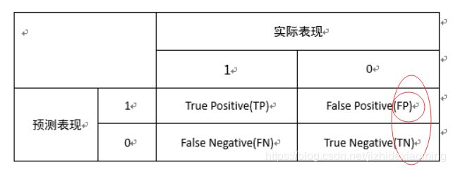
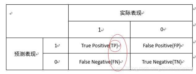
4. TP: 真正类，真实为正类，预测也为正类；

    FP: 假正类，真实为负类，预测为正类；

   TPR: 真正类率，TPR=TP/(TP+FN)，正确预测为正类占所有实际为正类样本的比例（所有实际为正类中被预测为正类的比例）；

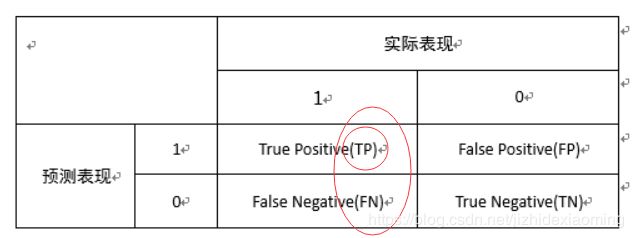
   FPR: 假正类率，FPR=FP/(FP+TN)，错误预测为正类占所有实际为负类样本的比例（实际为负类的样本中被预测为正类的比例）。

在显著性检测领域，生成的显著图的每个像素即为一个样本，显著图的像素按从大到小排序，然后从第一个（像素值最大）依次作为阈值，对所有像素进行分类，然后求得一组TPR, FPR。再以第二大的像素值为阈值，又可以得到一组。以FPR为横轴，以TPR为纵轴，即可得到ROC曲线，如下，ROC曲线的面积值即为AUC (area under curve)

5. 顺带提下准确率和召回率 （可以跳过）

Precision = TP/(TP+FP)，正确预测为正类的样本占所有预测为正类的比例，被预测为显著像素中实际为显著像素的比例

 Recall = TP/(TP+FN)，正确预测为正类的样本占所有实际为正类样本的比例，实际为显著像素中被预测（召回）为显著像素的比例，发现就是TPR

 

二，ROC和AUC值 

1，Matlab实现，算出auc = 0.8895，利用gongAUC_Judd.m，算出的auc = 0.8872

clear;
clc;

smap_full_path = strcat('D:\Code\Matlab\Map\smap.jpg');
gmap_full_path = strcat('D:\Code\Matlab\Map\gmap.jpg');
smap = imread(smap_full_path);
gmap = imread(gmap_full_path);

gmap = imresize(gmap,size(smap));
smap = imresize(smap,0.1);
gmap = imresize(gmap,0.1);

% 二值化ground truth map, 只要两类
thresh_value = graythresh(gmap);
final_gmap = im2bw(gmap, thresh_value);

% smap归一化到[0,1]
smap = mat2gray(smap);
% 
% [score,tp,fp,allthreshes] = AUC_Judd(smap, final_gmap, 1, 1);
% 数组
smap_array = smap(:); 
gmap_array = final_gmap(:);

% 总真实为正例数
idex = find(gmap_array == 1);
P_num = length(idex);

% 总真实为负例数
N_num = length(gmap_array) - P_num;

% 从大到小排序,orig_location保存了排序前像素在smap_array的位置
[saliency_values, orig_location] = sort(smap_array, 'descend'); 

% TP(1) = 0; FP(1) = 0; 
% TP(end) = 1; FP(end) = 1;
% 当以salicy_values(i)为阈值时，前面数组saliency_values前面i个都判为正例
for i=1:length(saliency_values)
    
    % 查看前i个被判为正例的像素，真实情况如何。
    TP(i) = 0; % 真正例，真实为正例，预测也为正例；
    FP(i) = 0; % 假正例，真实为负例，预测为正例；
    for m=1:i
        if gmap_array(orig_location(m)) == 1
            TP(i) = TP(i) + 1;
        else
            FP(i) = FP(i) + 1;
        end
    end
    
    FPR(i) = FP(i) / N_num;
    TPR(i) = TP(i) / P_num;
    
end

auc = trapz(FPR,TPR); % 以FPR为x轴，以TPR为y轴，算积分，即为ROC下的面积
plot(FPR, TPR, '.b-');   title(['Area under ROC curve: ', num2str(auc)])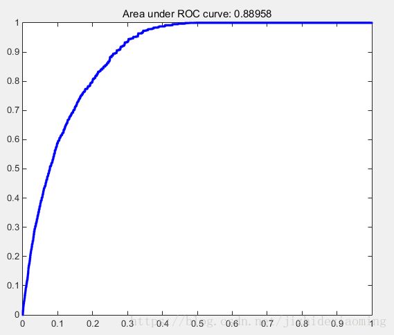

2， AUC_Judd.m

% created: Tilke Judd, Oct 2009
% updated: Zoya Bylinskii, Aug 2014

% This measures how well the saliencyMap of an image predicts the ground
% truth human fixations on the image. 

% ROC curve created by sweeping through threshold values 
% determined by range of saliency map values at fixation locations;
% true positive (tp) rate correspond to the ratio of saliency map values above 
% threshold at fixation locations to the total number of fixation locations
% false positive (fp) rate correspond to the ratio of saliency map values above 
% threshold at all other locations to the total number of posible other
% locations (non-fixated image pixels)

function [score,tp,fp,allthreshes] = AUC_Judd(saliencyMap, fixationMap, jitter, toPlot)
% saliencyMap is the saliency map
% fixationMap is the human fixation map (binary matrix)
% jitter = 1 will add tiny non-zero random constant to all map locations
% to ensure ROC can be calculated robustly (to avoid uniform region)
% if toPlot=1, displays ROC curve

if nargin < 4, toPlot = 0; end
if nargin < 3, jitter = 1; end
score = nan;

% If there are no fixations to predict, return NaN
if ~any(fixationMap)
    disp('no fixationMap');
    return
end 

if any(saliencyMap(:))
    saliencyMap = saliencyMap/sum(saliencyMap(:));
end

if any(fixationMap(:))
    fixationMap = fixationMap/sum(fixationMap(:));
end

% % make the saliencyMap the size of the image of fixationMap
% if size(saliencyMap, 1)~=size(fixationMap, 1) || size(saliencyMap, 2)~=size(fixationMap, 2)
%     saliencyMap = imresize(saliencyMap, size(fixationMap));
% end

% jitter saliency maps that come from saliency models that have a lot of
% zero values.  If the saliency map is made with a Gaussian then it does 
% not need to be jittered as the values are varied and there is not a large 
% patch of the same value. In fact jittering breaks the ordering 
% in the small values!
% if jitter
%     % jitter the saliency map slightly to distrupt ties of the same numbers
%     saliencyMap = saliencyMap+rand(size(saliencyMap))/10000000;
% end

% % normalize saliency map
% saliencyMap = (saliencyMap-min(saliencyMap(:)))/(max(saliencyMap(:))-min(saliencyMap(:)));
% 
% if sum(isnan(saliencyMap(:)))==length(saliencyMap(:))
%     disp('NaN saliencyMap');
%     return
% end

S = saliencyMap(:);
F = fixationMap(:);
   
Sth = S(F>0); % sal map values at fixation locations
Nfixations = length(Sth);
Npixels = length(S);

allthreshes = sort(Sth, 'descend'); % sort sal map values, to sweep through values
tp = zeros(Nfixations+2,1);
fp = zeros(Nfixations+2,1);
tp(1)=0; tp(end) = 1; 
fp(1)=0; fp(end) = 1;

for i = 1:Nfixations
    thresh = allthreshes(i);
    aboveth = sum(S >= thresh); % total number of sal map values above threshold
    tp(i+1) = i / Nfixations; % ratio sal map values at fixation locations above threshold
    fp(i+1) = (aboveth-i) / (Npixels - Nfixations); % ratio other sal map values above threshold
end 

score = trapz(fp,tp);
allthreshes = [1;allthreshes;0];

if toPlot
%     subplot(121); imshow(saliencyMap, []); title('SaliencyMap with fixations to be predicted');
%     hold on;
%     [y, x] = find(fixationMap);
%     plot(x, y, '.r');
%     subplot(122);
    plot(fp, tp, '.b-');   title(['Area under ROC curve: ', num2str(score)])
end

 

注：常用的显著性检测论文及代码汇总