numpy.polynomial 常见多项式操作

numpy.polynomial 常见多项式操作

构造一元多项式

函数: poly1d(c_or_r, r=False, variable=None)
输入：
c_or_r: 如果 r=False ，则 c_or_r 为: polynomial’s coefficients, in decreasing powers；如果 r=True，则 c_or_r 为: the polynomial’s roots. r默认为 False.
variable: 变量名
输出：
a one-dimensional polynomial class
示例：
1.如要根据系数序列构造多项式，构造多项式 $x^2+2x+3$：

a=np.poly1d([1,2,3],r=False,variable=["x"])

在命令输入:

2.根据多项式的根构造多项式:

a=np.poly1d([1,2,3],r=True,variable=["x"])

在命令输入:

a
Out[7]: poly1d([1, 2, 3])

多项式与数直接相乘和加减

以多项式 $a=x^2+2x+3$ 为例

5*a
Out[25]: poly1d([ 5, 10, 15])
a-5
Out[26]: poly1d([ 1,  2, -2])

快速求某点处的值

In[18]: a(0)
Out[18]: 3

poly1d 的 attributes

c=coef=coefficients=coeffs (系数): The polynomial coefficients

o =order(阶数): The order or degree of the polynomial

r =roots(根): The roots of the polynomial

variable(变量名): The name of the polynomial variable

print('系数:',a.c,\
'阶数:',a.order,\
'变量:',a.variable,\
'根:',a.r
)

输出

系数: [1 2 3] 阶数: 2 变量: x 根: [-1.+1.41421356j -1.-1.41421356j]

poly1d 的 Methods

例如求多项式 $2x+2$ 的积分和微分：

积分

a.integ(m=1,k=0)
poly1d([0.33333333, 1., 3., 0.])

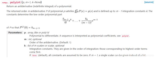
m : int, optional

Order of the antiderivative. (Default: 1)

k : list of m scalars or scalar, optional

Integration constants. They are given in the order of integration: those corresponding to highest-order terms come first.

微分：

a.deriv(m=1) 

m为阶数，即求几阶导数

多项式的四则运算

示例：

计算$x^2+2x+3$和$4x^2+5x+6$的和，差，积，商

polyadd(a1, a2) Find the sum of two polynomials.

polydiv(u, v) Returns the quotient and remainder of polynomial division.

polymul(a1, a2) Find the product of two polynomials.

polysub(a1, a2) Difference (subtraction) of two polynomials.

a=np.poly1d([1,2,3])
b=np.poly1d([4,5,6])

和

np.polyadd(a,b)
Out[31]: poly1d([5, 7, 9])

差

np.polysub(a,b)
Out[34]: poly1d([-3, -3, -3])

积

np.polymul(a,b)
Out[33]: poly1d([ 4, 13, 28, 27, 18])

商

np.polydiv(a,b)
Out[35]: (poly1d([0.25]), poly1d([0.75, 1.5 ]))

其中第一个是quotient，第二个是remainder

多项式的积分微分

积分

用法

np.polyint(a,m=2,k=[0,0])
Out[36]: poly1d([0.08333333, 0.33333333, 1.5, 0., 0.])

微分

np.polyder(a,m=1)# m为阶数
Out[38]: poly1d([2, 2])

多项式拟合

Least squares polynomial fit.

numpy.polyfit(x, y, deg, rcond=None, full=False, w=None, cov=False) Least squares polynomial fit.

输入参数

x: [array_like, shape (M,)] x-coordinates of the M sample points (x[i], y[i]).

y: [array_like, shape (M,) or (M, K)] y-coordinates of the sample points

deg(插值多项式阶数): Degree of the fitting polynomial

rcond [float, optional] : Relative condition number of the fit. Singular values smaller than this relative to the largest singular value will be ignored. The default value is len(x)*eps, where eps is the relative precision of the float type, about 2e-16 in most cases.

w(点的权重矩阵) [array_like, shape(M,), optional] : Weights to apply to the y-coordinates of the sample points. For gaussian uncertainties, use 1/sigma (not 1/sigma**2).

full [bool, optional] Switch determining nature of return value. When it is False (the default) just the coefficients are returned, when True diagnostic information from the singular value decomposition is also returned.

cov [bool or str, optional] If given and not False, return not just the estimate but also its covariance matrix. By default, the covariance are scaled by chi2/sqrt(N-dof), i.e., the weights are presumed to be unreliable except in a relative sense and everything is scaled such that the reduced chi2 is unity. This scaling is omitted if cov=‘unscaled’, as is relevant for the case that the weights are 1/sigma**2, with sigma known to be a reliable estimate of the uncertainty.

输出参数

p [ndarray, shape (deg + 1,) or (deg + 1, K)] : Polynomial coefficients, highest power first. If y was 2-D, the coefficients for k-th data set are in p[:,k].

residuals,rank,singular_values,rcond : Present only if full = True. Residuals of the least squares fit, the effective rank of the scaled Vandermonde coefficient matrix, its singular values, and the specified value of rcond.

V [ndarray, shape (M,M) or (M,M,K)] : Present only if full = False and cov‘=True. The covariance matrix of the polynomial coefficient estimates. The diagonal of this matrix are the variance estimates for each coefficient. If y is a 2-D array, then the covariance matrix for the ‘k-th data set are in V[:,:,k]

x = np.array([0.0, 1.0, 2.0, 3.0, 4.0, 5.0])
y = np.array([0.0, 0.8, 0.9, 0.1, -0.8, -1.0])
z = np.polyfit(x, y, 3)
z
# 结果 array([ 0.08703704, -0.81349206, 1.69312169, -0.03968254]) 

roots()——求根

多项式求根函数：roots(poly1d)

np.roots(a)
Out[20]: array([-1.+1.41421356j, -1.-1.41421356j])

polyval(p,x)——求值

计算多项式 p 在点 x 处的数值，等价于 p(x)

np.polyval(a,0.5)
Out[18]: 4.25`

ploy(sequence_of_roots)——根据根构造多项式

已知多项式的根写出多项式系数
$$y=(x-1)(x-2)(x-3)$$

构造多项式 y

np.poly([1,2,3])

结果：

array([ 1., -6., 11., -6.])