机器学习（吴恩达） python练习笔记第一周

一元线性回归方程：

from sklearn.linear_model import LinearRegression
import numpy as np
import matplotlib.pyplot as plt
import pandas as pd
from sklearn.model_selection import train_test_split

# 创建数据集
examDict = {'面积':[2000,2050,1000,980,500,520,400,450,300,200,100,1080,1520,580,900,1050,250],
            '价格':[1050,1000,520,520,260,270,220,240,140,110,60,500,780,280,450,510,125]}
examDf = pd.DataFrame(examDict)
# print(examDf)

# # 绘制散点图
# plt.scatter(examDf.面积 ,examDf.价格, color='b', label='Exam Data')
# # 添加图的标签（x轴，y轴）
# plt.xlabel('area')
# plt.ylabel('price')
# # plt.show()

# 相关系数R r(相关系数) = x和y的协方差/(x的标准差*y的标准差) == cov（x,y）/σx*σy（即person系数）
rDf = examDf.corr()
print(rDf)

# 将原始数据集拆分为训练集和测试集
exam_X = examDf.面积
exam_y = examDf.价格
X_train,X_test,y_train,y_test = train_test_split(exam_X, exam_y, train_size=.8, test_size=.2)
# print("原始数据特征:", exam_X.shape(), ",训练数据特征:", X_train.shape(), "测试数据特征：", X_test.shape())
# print("原始数据标签:", exam_y.shape(),",训练数据标签:",y_train.shape(),"测试数据标签：",y_test.shape())
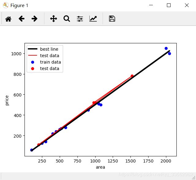
plt.scatter(X_train, y_train, color='b', label='train data')
plt.scatter(X_test, y_test, color='r', label='test data')
plt.legend(loc=2)
plt.xlabel('area')
plt.ylabel('price')
plt.savefig('tests.png')
# plt.show()

# 将训练集放入线性回归模型进行训练
lr = LinearRegression()
X_train = X_train.values.reshape(-1,1)
y_train = y_train.values.reshape(-1,1)
X_test = X_test.values.reshape(-1,1)
y_test = y_test.values.reshape(-1,1)
lr.fit(X_train,y_train)

a = lr.coef_ # 回归系数
b = lr.intercept_ # 截距
print("y=",a,"x+",b)

y_train_hat = lr.predict(X_train) # 训练数据的预测值
print("y_hat:",y_train_hat)
# 绘制拟合线
plt.plot(X_train, y_train_hat, color='black', linewidth=3, label='best line')
# 测试数据散点图
plt.plot(X_test, y_test, color='red', label='test data')
plt.legend(loc=2)
plt.xlabel('area')
plt.ylabel('price')
plt.savefig('lines.png')
plt.show()
print('测试集相关系数:', lr.score(X_test,y_test))


# 假设函数
def hypothesis(theta0, theta1, x):
    return theta1*x + theta0
# 代价函数
def Cost_Function(theta0, theta1, x, y):
    m = 4
    return 0.5/m * (np.square(theta1*x + theta0 - y)).sum()
# 优化函数
def optimize(theta0, theta1, x, y):
    m = 4
    alpha = 1
    y_hat = hypothesis(theta0, theta1, x)
    d_theta0 = 1/m * ((y_hat - y).sum())
    d_theta1 = 1/m * (((y_hat - y)*x).sum())
    theta0 = theta0 - alpha*d_theta0
    theta1 = theta1 - alpha*d_theta1
    return theta0, theta1

矩阵（单位阵，矩阵乘法，转置，求逆）：

import numpy as np

A = np.array([[1,2],[4,5]])
# A = np.reshape(A, newshape=(2,2))
B = np.array([[1,1],[0,2]])
# B = np.reshape(B, newshape=(2,2))
print(A)
print(B)
# 单位矩阵
I = np.eye(2)
print(I)
# 矩阵乘法：满足结合律不满足交换律
# dot为矩阵点乘，multiply为矩阵*乘即对应位置的元素相乘
IA = np.dot(I,A)
AI = np.dot(A,I)
AB = np.dot(A,B)
BA = np.dot(B,A)
print(IA)
print(AI)
print(AB)
print(BA)

C = np.array([[1,2,0], [0,5,6], [7,0,9]])
# A的转置矩阵
C_trans = C.T
print(C_trans)
# 矩阵的逆
C_inv = np.linalg.inv(C)
print(C_inv)
I = np.dot(C, C_inv)
# 设置输出矩阵的小数点位数
np.set_printoptions(formatter={'float':'{:0.2f}'.format})
print(I)

# transpose实现多维度变换
data = np.arange(24).reshape(2,3,4) # 2个3×4的矩阵
print(data)
print(data.transpose(1,0,2)) # 2,3,4三个参数分别对应0,1,2,交换后为3个2×4的矩阵
# swapaxes两轴对换
print(data.swapaxes(0,1)) # 实现2,3两个参数对换

多元线性回归方程

from sklearn.linear_model import LinearRegression
import numpy as np
import matplotlib.pyplot as plt
import pandas as pd
from sklearn.model_selection import train_test_split
# import seaborn as sn
# 创建数据集
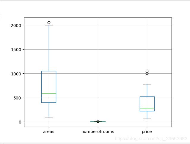
examDict = {'areas':[2000,2050,1000,980,500,520,400,450,300,200,100,1080,1520,580,900,1050,250],
            'numberofrooms':[10,10,5,4,3,3,2,3,2,1,1,5,7,3,4,5,1],
            'price':[1050,1000,520,520,260,270,220,240,140,110,60,500,780,280,450,510,125]}
examDf = pd.DataFrame(examDict)

# 得到所需要的数据集且查看前几列以及数据形状
print('head:', examDf.head())
# 数据描述
print(examDf.describe())
# 缺失值检验
print(examDf[examDf.isnull()==True].count())

examDf.boxplot()
plt.savefig('boxplot.png')
plt.show()

# 相关系数R r(相关系数) = x和y的协方差/(x的标准差*y的标准差) == cov（x,y）/σx*σy（即person系数）
print(examDf.corr())

# # 通过加入一个参数kind='reg'，seaborn可以添加一条最佳拟合直线和95%的置信带
# sns.pairplot(examDf, x_vars=['areas','number of rooms'], y_vars='price',size=7,aspect=0.8,kind='reg')
# plt.savefig("pairplot.png")
# plt.show()

# print(examDf.ix[:,:2])表示前两个特征
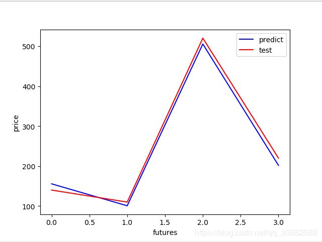
X_train, X_test, y_train, y_test = train_test_split(examDf.ix[:,:2], examDf.price, train_size=.8, test_size=.2)
lr = LinearRegression()
# X_train = X_train.values.reshape(-1,1)
# y_train = y_train.values.reshape(-1,1)
# X_test = X_test.values.reshape(-1,1)
# y_test = y_test.values.reshape(-1,1)
lr.fit(X_train, y_train)
print("回归系数：",lr.coef_,"/n截距：",lr.intercept_)
print("R方检测分数:",lr.score(examDf.ix[:,:2],examDf.price))

# 对先行回归进行预测
y_hat = lr.predict(X_test)
print("y_hat:",y_hat)

# 绘图
plt.figure()
plt.plot(range(len(y_hat)), y_hat, color='b', label='predict')
plt.plot(range(len(y_hat)), y_test, color='r', label='test')
plt.legend(loc='upper right')
plt.xlabel('futures')
plt.ylabel('price')
plt.savefig('predict.png')
plt.show()

参考文章：
https://blog.csdn.net/weixin_40014576/article/details/79918819#commentBox