GAM（广义相加模型）概要及R程序实现

国内关于GAM方面的资料不是一般的少，基本上都要往国外找。我光顾了没100都有50个网站，翻查了不少论文及资料，研究整理出下文，欢迎一同讨论。

GAM 广义相加模型Generalized additive model：

概念	回归模型中部分或全部的自变量采用平滑函数，降低线性设定带来的模型风险，对模型的假定不严，如不需要假定自变量线性相关于因变量（线性或非线性都可以）。 解决logistic回归当解释变量个数较多时容易引起维度灾难（Curse of dimensionality）。 光滑函数如应用到连续型解释变量。   * http://plantecology.syr.edu/fridley/bio793/gam.html
Equation	g is a link function, y independent, fi(xi)为光滑函数（未知），代替经典线性回归中的xi，对样本要求少，适用性广。（unspecified nonparametric function replaces a single coefficient）
估计方法	最小二乘法、likelyhood
检验	残差Pseduo系数(PCf)估计，PCf = 1 - RD / ND (RD残差偏差，ND 无效偏差)
分类	可加/非参数（Additive/Nonparametric）： 参数（Parametric）： 半参数/部分线性（Semiparametric/Partial Linear）： 薄板样条（Thin-plate spline）：, allow for interactions between two predictor
前提	如x1和x2并非独立而存在交互作用，则应设为Thin-plate spline: f(x1, x2) 模型中不必每一项都是非线性的，如都非线性会出现计算量大、过拟合等问题，通过查看xi与y的是否存在线性关系来判断是否使用平滑函数。 Should follow statistical and operational considerations.
光滑函数	见“样条函数”
缺点	样条函数不定参使之不能直接用于预估新的数据（Lack of parametric functional form makes it difficult to score the new data directly）
Q&A	How to define smooth.terms in R.mgcv.GAM? competing philosophies: from "Try everything and go with the one that produces the best fit" (as measured by something like AIC) to "Write the one model that best reflects your understanding of the data-generating process and use it."

广义交叉验证法（GCV，generalized cross-validation）

基本原理是当式Ax=b的测量值 b 中的任意一项i b被移除时，所选择的正则参数应能预测到移除项所导致的变化。

 

马洛斯的Cp、Cp—准则（Mallows' Cp）

用来帮助在多个候选回归模型之间进行选择的一个统计量。Cp＝(SSEp)/(2)-(n-2p)。

注：仅当使用相同的预测变量时，使用Mallows Cp 比较回归模型才有效。

结合Scorecard

S0 = Intercept (only forBernoulli Likelihood objective function)

c1,c2, ..., cp = Scorecardcharacteristics

S1,S2,...,Sq = Score weightsassociated with the bins of a characteristics

X1,X2,...,Xq= Dummy indicatorvariables for the bins of a characteristics

关键是Score Weight的设定。

Y的分布	联系函数名称	f(Y)
正态分布（normal）	Identity	Y
二项分布（binomial）	Logit	Logit（Y）
Poisson分布	Log	Log（Y）
γ 分布（gamma）	inverse	1/（Y-1）
负二项分布（negative binomial）	Log	Log（Y）

样条函数（spline function）

概念：早期工程师制图时，把富有弹性的细长木条（所谓样条）用压铁固定在样点上，在其他地方让它自由弯曲，然后沿木条画下曲线。成为样条曲线。

分段光滑、并且在各段交接处也有一定光滑性的函数，具有较好的数值稳定性和收敛性。

可多次样条，最常用是二次和三次样条。

 

（1）三次样条插值（Cubic smoothingspline）

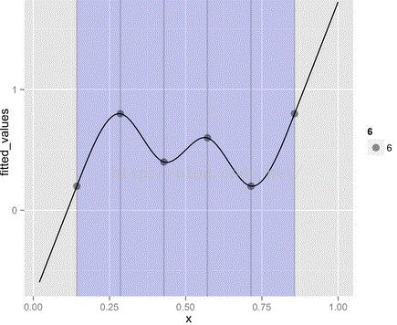
定义:函数S(x)∈C2[a,b] ，且在每个小区间[ xj,xj+1 ]上是三次多项式，其中a =x0

. To the left of the sequence of knots, anatural cubic spline is a line.

. Between knots, a natural cubic spline isa third degree polynomial curve. Hence the cubic in the name.

. At the knots, the curve must becontinuous. At the knots, the derivative also must be continuous (no corner).At the knots, the second derivative must be continuous.

（2）cyclic spline

Live on a "circle", e.g. theytake values in the interval [0,1), and 0=1. like cyclic cubic regressionspline, cyclic p-spline.

R程序：

Concept	Separate cubic polynomials are fit at each section, and then joined at the knots to create a continuous curve. effective degrees of freedom, or edf. In typical OLS regression the model degrees of freedom is equivalent to the number of predictors/terms in the model. s(Girth,Height)  #Girth 和 Height 不独立，存在相互影响 gam(Overall ~ Income + Edu + Health, data = d)  # 此时与glm一样 smooth terms: 其实就是应用了光滑函数的自变量e.g. s(agecont), te(Month,Age)   l  http://www.rdocumentation.org/packages/mgcv/functions/gam
gam syntax	gam(y~s(x,k = , bs =)) / gam(y~te(x,k = , bs =)) Choose.k: sets up the dimensionality of the smoothing matrix for each term. Penalized regression smoothers. Using a substantially increased k to see if there is pattern in the residuals that could potentially be explained by increasing k. Default任意数字（normally 10 degree of freedom）。 bs: See smooth.terms for the full list. tp – DEFAULT, thin plate regression spline,cr – penalized cubic regression spline三次样条, cs – shrinkage version of cr,cc – cyclic cubic regression spline, ps – P-spline,cp – cyclic p-spline, ad – adaptive smoothing, fs – factor smooth interaction. s: smooth s(covariate, edf); te: tensor product smooth   gam(formula,family=gaussian(),data=list(),weights=NULL,subset=NULL,   na.action,offset=NULL,method="GCV.Cp",   optimizer=c("outer","newton"),control=list(),scale=0,   select=FALSE,knots=NULL,sp=NULL,min.sp=NULL,H=NULL,gamma=1,   fit=TRUE,paraPen=NULL,G=NULL,in.out,...) offset: Can be used to supply a model offset for use in fitting. Note that this offset will always be completely ignored when predicting, unlike an offset included in formula. control: A list of fit control parameters to replace defaults returned by gam.control. method: smoothing parameter estimation method. e.g. "GCV.Cp", "GACV.Cp", "REML", "P-REML", "ML", "P-ML" (ML = maximum likelihood, REML = 约束性最大似然法 restricted maximum likelihood) fit: If this argument is TRUE then gam sets up the model and fits it, but if it is FALSE then the model is set up and an object G containing what would be required to fit is returned is returned. Gamma: multiplier to inflate the degrees of freedom in the GCV/UBRE/AIC score. Select: TRUE means adding an extra penalty to each term so that it can be penalized to zero.   s(x1, by=x2) e.g. Loc = America, Doy = as.numeric(format(Date,format = "%j")), s(Doy,by = Loc)
test	gam.check(b)  # k' = k - 1 summary(gammodel) (1) GCV, with lower being better. (2) R-sq.(adj) near to 1 is better. AIC(mod_1d, mod_2d) (3) with lower being better. anova(b)  # Wald like tests anova(mod_1d, mod_2d, test = "Chisq")  #取lower resid.deviance anova(b,b1,test="F") (4) select the significant one
plot	plot(mod_gam2, pages=1, residuals=T, shade=T, col='#FF8000') vis.gam(mod_gam2, type = "response", plot.type = "contour") vis.gam(mod_gam2, type = "response", plot.type = "persp", border=NA, phi=30, theta=30) * If the graph looks noise, then the smooth function may be not suitable. * http://stats.stackexchange.com/questions/14746/what-does-the-dashed-bounds-mean-when-plotting-a-contour-plot-with-r-gam
Q&A	Err: - not meaningful for factors in: Ops.factor(xx, shift[i]) A: smoothing a factor, which isn't supported (`smooth' means that f(x_1) must be close to f(x_2), e.g. if a factor has levels "brick", "sky" and "purple", how far is it from "brick" to "purple"?)   Err: A term has fewer unique covariate combinations than specified maximum degrees of freedom / basis dimension is larger than number of unique covariates A: for smoothing function, one independent variables portfolio cannot match to different response variable values.   Q: how to choose a proper smoothing spline (bs='?') A: 1) use the default; 2) use a tensor product of "cr" smooths for bivariate smoothing, ie. te=(x,bs=”cr”)
Summary	Formula: LN_Brutto ~ s(agecont, by = Sex) + factor(Sex) + te(Month, Age) +     s(Month, by = Sex)   Parametric coefficients:              Estimate Std. Error t value Pr(>|t|)    (Intercept)   4.32057    0.01071  403.34   <2e-16 *** factor(Sex)m  0.27708    0.01376   20.14   <2e-16 *** --- Signif. codes:  0 '***' 0.001 '**' 0.01 '*' 0.05 '.' 0.1 ' ' 1   Approximate significance of smooth terms:                     edf  Ref.df      F  p-value    s(agecont):Sexf  8.1611  8.7526 20.170  < 2e-16 *** s(agecont):Sexm  6.6695  7.5523 32.689  < 2e-16 *** te(Month,Age)   10.3651 12.7201  6.784 2.19e-12 *** s(Month):Sexf    0.9701  0.9701  0.641    0.430    s(Month):Sexm    1.3750  1.6855  0.193    0.787    --- Signif. codes:  0 '***' 0.001 '**' 0.01 '*' 0.05 '.' 0.1 ' ' 1   Rank: 60/62 R-sq.(adj) =  0.781   Deviance explained = 78.7% GCV = 0.048221  Scale est. = 0.046918  n = 1093