SLAM从入门到放弃：SLAM十四讲第十三章习题（2-3）

以下均为简单笔记，如有错误，请多多指教。

2. 把本讲的稠密深度估计改成半稠密，你可以先把梯度明显的地方筛选出来。
3. 把本讲演示的单目稠密重建代码从正深度改成逆深度，并添加仿射变换。你的实验效果是否有改进？
   解：此处把两个题目的解放在一起，以下就是所有的代码，将分别注释相关的代码。
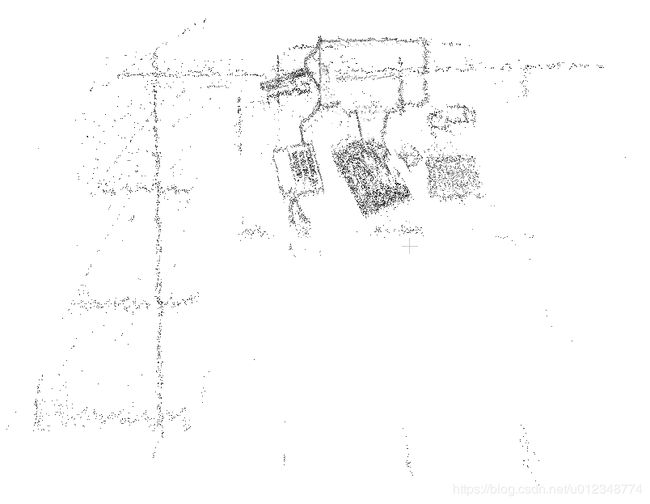
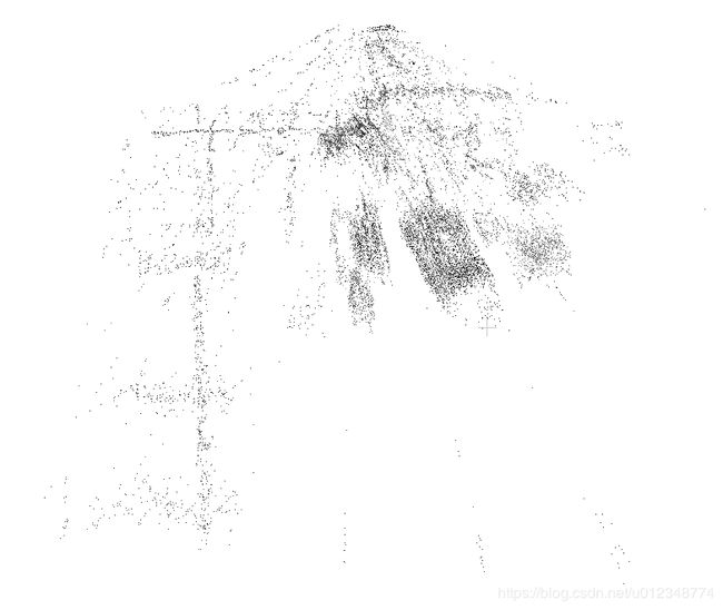
   以下是经过代码更新后的点云图和原始的点云图，可以发现更新后质量明显更高。
   
   

#include 
#include 
#include 
using namespace std; 
#include 

// for sophus 
#include 
using Sophus::SE3;

// for eigen 
#include 
#include 
using namespace Eigen;

#include 
#include 
#include 

using namespace cv;

/**********************************************
* 本程序演示了单目相机在已知轨迹下的稠密深度估计
* 使用极线搜索 + NCC 匹配的方式，与书本的 13.2 节对应
* 请注意本程序并不完美，你完全可以改进它——我其实在故意暴露一些问题。
***********************************************/



// ------------------------------------------------------------------
// parameters 
const int boarder = 20; 	// 边缘宽度
const int width = 640;  	// 宽度 
const int height = 480;  	// 高度
const double fx = 481.2f;	// 相机内参
const double fy = -480.0f;
const double cx = 319.5f;
const double cy = 239.5f;
const int ncc_window_size = 2;	// NCC 取的窗口半宽度
const int ncc_area = (2*ncc_window_size+1)*(2*ncc_window_size+1); // NCC窗口面积
const double min_cov = 0.001;	// 收敛判定：最小方差
const double max_cov = 0.5;	// 发散判定：最大方差

// ------------------------------------------------------------------
// 重要的函数 
// 从 REMODE 数据集读取数据  
bool readDatasetFiles( 
    const string& path, 
    vector& color_image_files, 
    vector& poses 
);

// 根据新的图像更新深度估计
bool update( 
    const Mat& ref, 
    const Mat& curr, 
    const SE3& T_C_R, 
    Mat& depth, 
    Mat& depth_cov 
);

// 极线搜索 
bool epipolarSearch( 
    const Mat& ref, 
    const Mat& curr, 
    const SE3& T_C_R, 
    const Vector2d& pt_ref, 
    const double& depth_mu, 
    const double& depth_cov,
    Vector2d& pt_curr
);

// 更新深度滤波器 
bool updateDepthFilter( 
    const Vector2d& pt_ref, 
    const Vector2d& pt_curr, 
    const SE3& T_C_R, 
    Mat& depth, 
    Mat& depth_cov
);

// 计算 NCC 评分 
double NCC( const Mat& ref, const Mat& curr, const Vector2d& pt_ref, double depth, Vector2d& pt_cur, const SE3& T_C_R );

// 双线性灰度插值 
inline double getBilinearInterpolatedValue( const Mat& img, const Vector2d& pt ) {
    uchar* d = & img.data[ int(pt(1,0))*img.step+int(pt(0,0)) ];
    double xx = pt(0,0) - floor(pt(0,0)); 
    double yy = pt(1,0) - floor(pt(1,0));
    return  (( 1-xx ) * ( 1-yy ) * double(d[0]) +
            xx* ( 1-yy ) * double(d[1]) +
            ( 1-xx ) *yy* double(d[img.step]) +
            xx*yy*double(d[img.step+1]))/255.0;
}

// ------------------------------------------------------------------
// 一些小工具 
// 显示估计的深度图 
void plotDepth( const Mat& depth );

// 像素到相机坐标系 
inline Vector3d px2cam ( const Vector2d px ) {
    return Vector3d ( 
        (px(0,0) - cx)/fx,
        (px(1,0) - cy)/fy, 
        1
    );
}

// 相机坐标系到像素 
inline Vector2d cam2px ( const Vector3d p_cam ) {
    return Vector2d (
        p_cam(0,0)*fx/p_cam(2,0) + cx, 
        p_cam(1,0)*fy/p_cam(2,0) + cy 
    );
}

// 检测一个点是否在图像边框内
inline bool inside( const Vector2d& pt ) {
    return pt(0,0) >= boarder && pt(1,0)>=boarder 
        && pt(0,0)+boarder color_image_files; 
    vector poses_TWC;
    bool ret = readDatasetFiles( argv[1], color_image_files, poses_TWC );
    if ( ret==false )
    {
        cout<<"Reading image files failed!"<(y)[x] > min_cov  ) // 深度已收敛或发散
                continue;
            
            Vector3d f_ref = px2cam( Vector2d(x,y) );
            f_ref.normalize();
            Vector3d P_ref = f_ref*depth.ptr(y)[x];	// 参考帧的 P 向量

            points<(y)[x])<<"\t"<(y)[x])<<"\t"<(y)[x])<<"\t"<& color_image_files, 
    std::vector& poses
)
{
    ifstream fin( path+"/first_200_frames_traj_over_table_input_sequence.txt");
    if ( !fin ) return false;
    
    while ( !fin.eof() )
    {
		// 数据格式：图像文件名 tx, ty, tz, qx, qy, qz, qw ，注意是 TWC 而非 TCW
        string image; 
        fin>>image; 
        double data[7];
        for ( double& d:data ) fin>>d;
        
        color_image_files.push_back( path+string("/images/")+image );
        poses.push_back(
            SE3( Quaterniond(data[6], data[3], data[4], data[5]), 
                 Vector3d(data[0], data[1], data[2]))
        );
        if ( !fin.good() ) break;
    }
    return true;
}

// 对整个深度图进行更新
bool update(const Mat& ref, const Mat& curr, const SE3& T_C_R, Mat& depth, Mat& depth_cov )
{
#pragma omp parallel for
    for ( int x=boarder; x(y)[x+1] - ref.ptr(y)[x-1], 
                        ref.ptr(y+1)[x] - ref.ptr(y-1)[x]
                    );
            // 把梯度小的区域过滤到
            if ( delta.norm() < 50 )
                continue;

	        // 遍历每个像素
            if ( depth_cov.ptr(y)[x] < min_cov || depth_cov.ptr(y)[x] > max_cov ) // 深度已收敛或发散
                continue;
            // 在极线上搜索 (x,y) 的匹配 
            Vector2d pt_curr; 
            bool ret = epipolarSearch ( 
                ref, 
                curr, 
                T_C_R, 
                Vector2d(x,y), 
                depth.ptr(y)[x], 
                sqrt(depth_cov.ptr(y)[x]),
                pt_curr
            );
            
            if ( ret == false ) // 匹配失败
                continue; 
            
			// 取消该注释以显示匹配
            // showEpipolarMatch( ref, curr, Vector2d(x,y), pt_curr );
            
            // 匹配成功，更新深度图 
            updateDepthFilter( Vector2d(x,y), pt_curr, T_C_R, depth, depth_cov );
        }
}

// 极线搜索
// 方法见书 13.2 13.3 两节
bool epipolarSearch(
    const Mat& ref, const Mat& curr, 
    const SE3& T_C_R, const Vector2d& pt_ref, 
    const double& depth_mu, const double& depth_cov, 
    Vector2d& pt_curr )
{
    // 此处是为逆深度做准备
    // 因此需要根据方差求解出逆深度的范围
    double d_min = 1/depth_mu-3*depth_cov, d_max = 1/depth_mu+3*depth_cov;
    // 防止小于0
    if(d_min<0) d_min = 0.2;
    // 求出深度范围
    double dd_max = 1/d_min;
    double dd_min = 1/d_max;
    if ( dd_min<0.1 ) dd_min = 0.1;
    
    // 在极线上搜索，以深度均值点为中心，左右各取半长度
    double best_ncc = -1.0;
    Vector2d best_px_curr; 
    for ( double l=dd_min; l<=dd_max; l+=0.1 )  // l+=sqrt(2) 
    {
        // 计算待匹配点与参考帧的 NCC
        Vector2d px_curr; 
        // 此处是增加了放射变换的NCC计算
        double ncc = NCC( ref, curr, pt_ref, l, px_curr, T_C_R);
        if ( ncc>best_ncc )
        {
            best_ncc = ncc; 
            best_px_curr = px_curr;
        }
    }
    if ( best_ncc < 0.85f )      // 只相信 NCC 很高的匹配
        return false; 
    pt_curr = best_px_curr;
    return true;
}

double NCC (
    const Mat& ref, const Mat& curr, 
    const Vector2d& pt_ref, double depth,
    Vector2d& pt_cur,
    const SE3& T_C_R 
)
{
    // 零均值-归一化互相关
    // 先算均值
    double mean_ref = 0, mean_curr = 0;
    vector values_ref, values_curr; // 参考帧和当前帧的均值
    // 以下代码中又进行放射变换计算的代码
    // 其核心思路是假设参考影像上一点附近都为一个平面且深度都一样
    for ( int x=-ncc_window_size; x<=ncc_window_size; x++ )
        for ( int y=-ncc_window_size; y<=ncc_window_size; y++ )
        {
            // 从像平面坐标系到像空间坐标系
            Vector2d pointRef(int(x+pt_ref(0,0)),int(y+pt_ref(1,0)));
            Vector3d f_ref = px2cam( pointRef );
            f_ref.normalize();
            
            double value_ref = double(ref.ptr( int(pointRef(1,0)) )[ int(pointRef(0,0)) ])/255.0;
            mean_ref += value_ref;
            
            // 根据放射变换算出到参考影像上的坐标
            Vector3d P_ref = f_ref*depth;	// 参考帧的 P 向量
            Vector2d px_curr = cam2px( T_C_R*P_ref ); // 按深度均值投影的像素

            if( x==0 && y==0 )
            {
                pt_cur = px_curr;
            }

            if ( !inside(px_curr) )
                return -1.0; 

            double value_curr = getBilinearInterpolatedValue( curr, px_curr );
            mean_curr += value_curr;
            
            values_ref.push_back(value_ref);
            values_curr.push_back(value_curr);
        }
        
    mean_ref /= ncc_area;
    mean_curr /= ncc_area;
    
	// 计算 Zero mean NCC
    double numerator = 0, demoniator1 = 0, demoniator2 = 0;
    for ( int i=0; i [ f_ref^T f_ref, -f_ref^T f_cur ] [d_ref] = [f_ref^T t]
    //    [ f_cur^T f_ref, -f_cur^T f_cur ] [d_cur] = [f_cur^T t]
    // 二阶方程用克莱默法则求解并解之
    Vector3d t = T_R_C.translation();
    Vector3d f2 = T_R_C.rotation_matrix() * f_curr; 
    Vector2d b = Vector2d ( t.dot ( f_ref ), t.dot ( f2 ) );
    double A[4];
    A[0] = f_ref.dot ( f_ref );
    A[2] = f_ref.dot ( f2 );
    A[1] = -A[2];
    A[3] = - f2.dot ( f2 );
    double d = A[0]*A[3]-A[1]*A[2];
    Vector2d lambdavec = 
        Vector2d (  A[3] * b ( 0,0 ) - A[1] * b ( 1,0 ),
                    -A[2] * b ( 0,0 ) + A[0] * b ( 1,0 )) /d;
    Vector3d xm = lambdavec ( 0,0 ) * f_ref;
    Vector3d xn = t + lambdavec ( 1,0 ) * f2;
    Vector3d d_esti = ( xm+xn ) / 2.0;  // 三角化算得的深度向量
    double depth_estimation = d_esti.norm();   // 深度值
    
    // 计算不确定性（以一个像素为误差）
    Vector3d p = f_ref*depth_estimation;
    Vector3d a = p - t; 
    double t_norm = t.norm();
    double a_norm = a.norm();
    double alpha = acos( f_ref.dot(t)/t_norm );
    double beta = acos( -a.dot(t)/(a_norm*t_norm));
    double beta_prime = beta + atan(1/fx);
    double gamma = M_PI - alpha - beta_prime;
    double p_prime = t_norm * sin(beta_prime) / sin(gamma);
 
   // 逆深度的方差更新方式
    double d_cov = 1/p_prime - 1/depth_estimation; 
    double d_cov2 = d_cov*d_cov;
    
    // 高斯融合
    double mu = depth.ptr( int(pt_ref(1,0)) )[ int(pt_ref(0,0)) ];
    double sigma2 = depth_cov.ptr( int(pt_ref(1,0)) )[ int(pt_ref(0,0)) ];

    double mu_fuse = (d_cov2/mu+sigma2/depth_estimation) / ( sigma2+d_cov2);
    double sigma_fuse2 = ( sigma2 * d_cov2 ) / ( sigma2 + d_cov2 );
    
    depth.ptr( int(pt_ref(1,0)) )[ int(pt_ref(0,0)) ] = 1/mu_fuse; 
    depth_cov.ptr( int(pt_ref(1,0)) )[ int(pt_ref(0,0)) ] = sigma_fuse2;

    
    return true;
}

// 后面这些太简单我就不注释了（其实是因为懒）
void plotDepth(const Mat& depth)
{
    imshow( "depth", depth*0.4 );
    waitKey(1);
}