Mnist数据集测试demo
参考tensorflow官网中的demo:mnist
分析mnist的数据集的格式:
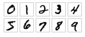
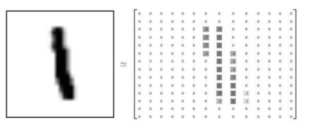
28*28的矩阵格式,1表示该像素点为黑,0代表该像素点为白
然后,导入数据集:
import tensorflow as tf
import tensorflow.examples.tutorials.mnist.input_data as input_data
mnist = input_data.read_data_sets("MNIST_data/", one_hot=True)
设置占位符:
因为28*28 = 784 所以每次塞入的数据是784个
x = tf.placeholder(tf.float32, [None, 784])#输入的数据占位符
y_actual = tf.placeholder(tf.float32, shape=[None, 10])#输入的标签占位符
权重和偏置初始化函数
权重使用的truncated_normal进行初始化,stddev标准差定义为0.1
偏置初始化为常量0.1:
'''权重初始化函数'''
def weight_variable(shape): inital = tf.truncated_normal(shape, stddev=0.1) # 使用truncated_normal进行初始化
return tf.Variable(inital)
'''偏置初始化函数'''
def bias_variable(shape): inital = tf.constant(0.1,shape=shape)
# 偏置定义为常量
return tf.Variable(inital)
卷积函数
strides[0]和strides[3]的两个1是默认值,中间两个1代表padding时在x方向运动1步,y方向运动1步
padding='SAME'代表经过卷积之后的输出图像和原图像大小一样
#定义一个函数,用于构建卷积层
def conv2d(x, W):
return tf.nn.conv2d(x, W, strides=[1, 1, 1, 1], padding='SAME')
定义池化函数:
def max_pool(x):
return tf.nn.max_pool(x, ksize=[1, 2, 2, 1],strides=[1, 2, 2, 1], padding='SAME')
构建网络:
#构建网络
x_image = tf.reshape(x, [-1,28,28,1]) #转换输入数据shape,以便于用于网络中
W_conv1 = weight_variable([5, 5, 1, 32])
b_conv1 = bias_variable([32])
h_conv1 = tf.nn.relu(conv2d(x_image, W_conv1) + b_conv1) #第一个卷积层
h_pool1 = max_pool(h_conv1) #第一个池化层
W_conv2 = weight_variable([5, 5, 32, 64])
b_conv2 = bias_variable([64])
h_conv2 = tf.nn.relu(conv2d(h_pool1, W_conv2) + b_conv2) #第二个卷积层
h_pool2 = max_pool(h_conv2) #第二个池化层
W_fc1 = weight_variable([7 * 7 * 64, 1024])
b_fc1 = bias_variable([1024])
h_pool2_flat = tf.reshape(h_pool2, [-1, 7*7*64]) #reshape成向量
h_fc1 = tf.nn.relu(tf.matmul(h_pool2_flat, W_fc1) + b_fc1) #第一个全连接层
keep_prob = tf.placeholder("float")
h_fc1_drop = tf.nn.dropout(h_fc1, keep_prob) #dropout层
W_fc2 = weight_variable([1024, 10])
b_fc2 = bias_variable([10])
y_predict=tf.nn.softmax(tf.matmul(h_fc1_drop, W_fc2) + b_fc2) #softmax层
开始训练:
cross_entropy = -tf.reduce_sum(y_actual*tf.log(y_predict)) #交叉熵
train_step = tf.train.GradientDescentOptimizer(1e-3).minimize(cross_entropy) #梯度下降法
correct_prediction = tf.equal(tf.argmax(y_predict,1), tf.argmax(y_actual,1))
accuracy = tf.reduce_mean(tf.cast(correct_prediction, "float")) #精确度计算
sess=tf.InteractiveSession()
sess.run(tf.initialize_all_variables())
for i in range(20000):
batch = mnist.train.next_batch(50)
if i%100 == 0: #训练100次,验证一次
train_acc = accuracy.eval(feed_dict={x:batch[0], y_actual: batch[1], keep_prob: 1.0})
print 'step %d, training accuracy %g'%(i,train_acc)
train_step.run(feed_dict={x: batch[0], y_actual: batch[1], keep_prob: 0.5})
test_acc=accuracy.eval(feed_dict={x: mnist.test.images, y_actual: mnist.test.labels, keep_prob: 1.0})
print("test accuracy",test_acc)
运行结果:
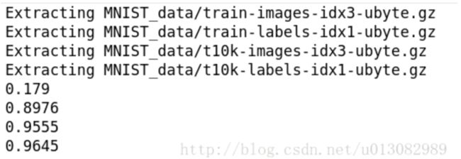
效果还算不错。