概率论与随机过程笔记（1）：样本空间与概率

概率论与随机过程笔记（1）：样本空间与概率

2019-10-27

---

这部分的笔记依据Dimitri P. Bertsekas和John N. Tsitsiklis的《概率导论》第1章内容（不包括1.6节组合数学的内容）。鉴于线性代数的笔记中大量latex公式输入中，切换中英文输入法浪费了很多时间，所以概率笔记会用英文完成。

1.1 集合（sets）

【集合的定义】A set is a collection of objects, which are the elements of the set. If $S$ is a set and $x$ is an element of $S$, we write $x\in S$. If $x$ is not an element of $S$, we write $x\notin S$. A set can have no elements, in which case it is called the empty set, denoted by $\varnothing$

【集合的表示方法】Sets can be specified in a variety of ways:
$$S=\{x_1,x_2,\cdots ,x_n\}$$$$S=\{x_1,x_2,\cdots \}$$$$\{x|xsatisfiesP\}$$
The symbol “$|$” is to be read as “such that.”

【集合之间的关系】If every element of a set $S$ is also an element of a set $T$, we say that $S$ is a subset of $T$, and we write $S\subset T$ or $T\supset S$. If $S\subset T$ and $T\subset S$, the two sets are equal, and we write $S=T$.

【空间 $\Omega$】It is also expedient to introduce a universal set, denoted by $\Omega$, which contains all objects that could conceivably be of interest in a particular context. Having specified the context in terms of a universal set $\Omega$, we only consider sets $S$ that are subsets of $\Omega$.

【补集】The complement of a set $S$, with respect to the universe $\Omega$, is the set $\{x\in \Omega |x\notin S\}$ of all the elements of $\Omega$ that do not belong to $S$, and is denoted by $S^c$. Note that ${\Omega }^c=\varnothing$.

【集合的交和并】The union of two sets $S$ and $T$ is the set of all elements that belong to $S$ or $T$ (or both), and is denoted by $S\cup T$. The intersection of two sets $S$ and $T$ is the set of all elements that belong to both $S$ and $T$, and is denoted by $S\cap T$. Thus, $$S\cup T=\{x|x\in Sorx\in T\}$$ $$S\cap T=\{x|x\in Sandx\in T\}$$ $$\bigcup _{n=1}^{\infty }=S_1\cup S_2\cdots =\{x|x\in S_{n}forsomen\}$$ $$\bigcap _{n=1}^{\infty }=S_1\cap S_2\cdots =\{x|x\in S_{n}forallen\}$$
【不想交 & 分割】Two sets are said to be disjoint if their intersection is empty. More generally, several sets are said to be disjoint if no two of them have a common element. A collection of sets is said to be a partition of a set $S$ if the sets in the collection are disjoint and their union is $S$.

If $x$ and $y$ are two objects. we use $(x.y)$ to denote the ordered pair of $x$ and $y$. The set of scalars (real numbers) is denoted by $\mathbb{R}$: the set of pairs (or triplets) of scalars, i.e … the two-dimensional plane (or three-dimensional space, respectively) is denoted by ${\mathbb{R}}^2$ (or ${\mathbb{R}}^3$. respectively).

Sets and the associated operations are easy to visualize in terms of Venn diagrams. as illustrated in Fig. 1.1.

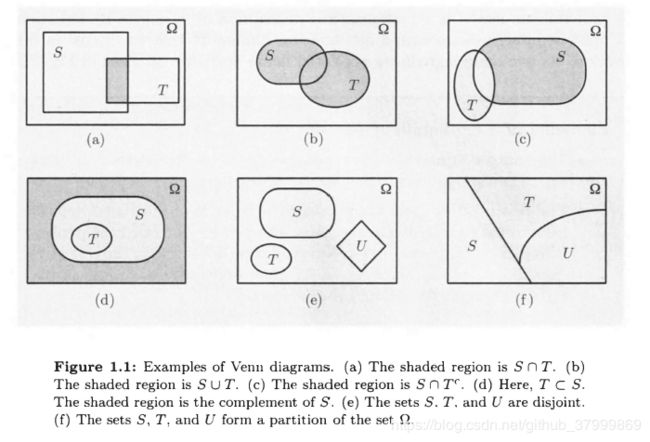
【矩阵代数】Set operations have several properties, which are elementary consequences of the definitions. Some exa1nples are:

• $S\cup T=T\cup S$
• $S\cup (T\cup U)=(S\cup T)\cup U$
• $S\cap (T\cup U)=(S\cap T)\cup (S\cap U)$
• $S\cup (T\cap U)=(S\cup T)\cap (S\cup U)$
• $(S^c{)}^c=S$
• $S\cap S^c=\varnothing$
• $S\cup \Omega =\Omega$
• $S\cap \Omega =S$

Two particularly useful properties are given by De Morgan’s laws which state that:$$(\bigcup _n{S}_n{)}^c=\bigcap _n{S}_n^c$$ $$(\bigcap _n{S}_n{)}^c=\bigcup _n{S}_n^c$$

1.2 概率模型（probablistic models）

A probabilistic model is a mathematical description of an uncertain situation.Its two main ingredients are listed below and are visualized in Fig. 1.2.

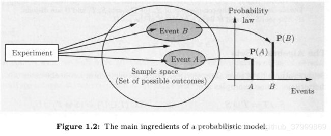
Elements of a Probabilistic Model：

• The sample space $\Omega$, which is the set of all possible outcomes of an experiment.
• The probability law, which assigns to a set $A$ of possible outcomes (also called an event) a nonnegative number $P(A)$ (called the probability of $A$) that encodes our knowledge or belisf about the collective “likelihood” of the elements of $A$.

【样本空间和事件】Every probabilistic model involves an underlying process, called the experiment, that will produce exactly one out of several possible outcomes. The set of all possible outcomes is called the sample space of the experiment, and is denoted by $\Omega$. A subset of the sample space, that is, a collection of possible outcomes, is called an event. here is no restriction on what constitutes an experiment.
The sample space of an experiment may consist of a finite or an infinite number of possible outcomes. Finite sample spaces are conceptually and mathematically simpler.
Generally, the sample space chosen for a probabilistic model must be collectively exhaustive, in the sense that no matter what happens in the experiment, we always obtain an outcome that has been included in the sample space. In addition, the sample space should have enough detail to distinguish between all outcomes of interest to the modeler, while avoiding irrelevant details.

【概率律（probability law.）】the probabilitylaw assigns to every event $A$. a number $P(A)$, called the probability of $A$. satisfying the following axioms:

• (Nonnegativity) $P(A)\ge 0$, for every event $A$
• (Additivity) If $A$ and $B$ are two disjoint events, then the probability of their union satisfies $$P(A\cup B)=P(A)+P(B)$$. More generally, if the sample space has an infinite number of elements and $A_1$, $A_2$, $\cdots$ is a sequence of disjoint events, then the probability of their union satifies $$P(A_1\cup A_2\cup \cdots )=P(A_1)+P(A_2)+\cdots$$
• (Normalization) The probability of the entire sample space $\Omega$ is equal to 1, that is, $P(\Omega )=1$

【离散概率律（Discrete Probability Law）】If the sample space consists of a finite number of possible outcomes, then the probability law is specified by the probabilities of the events that consist of a single element. In particular, the probability of any event $\{s_1,s_2,\cdots ,s_n\}$ is the sum of the probabilities of its elements: $$P(\{s_1,s_2,\cdots ,s_n\})=P(s_1)+P(s_2)+\cdots +P(s_n)$$

【离散均匀概率律（古典模型）（Discrete Uniform Probability Law）】In the special case where the probabilities $P(s_1),\cdots ,P(s_n)$ are all the same (by necessity equal to $1/n$, in view of the normalization axiom). If the sample space consists of n possible outcomes which are equally likely (i.e, all single-element events have he same probability), then the probability of any event $A$ is given by $$P(A)=\frac{numberofelementsofA}{n}$$

【连续模型】Probabilistic models with continuous sample spaces differ from their discrete counterparts in that the probabilities of the single-element events may not be sufficient to characterize the probability law. This is illustrated in the following examples, which also indicate how to generalize the uniform probability law to the case of a continuous sample space.

A wheel of fortune is continuously calibrated from 0 to 1, so the possible outcomes of an experiment consisting of a single spin are the numbers in the interval $n=[0,1]$. Assuming a fair wheel, it is appropriate to consider all outcomes equally likely, but what is the probability of the event consisting of a single element? It cannot be positive, because then, using the additivity axiom, it would follow that events with a sufficiently large number of elements would have probability larger than 1. Therefore, the probability of any event that consists of a single element must be 0.
In this example, it makes sense to assign probability $b-a$ to any subinterval $[a,b]$ of $[0,1]$, and to calculate the probability of a more complicated set by evaluating its “length”. (${\int }_{S}dt$) This assignment satisfies the three probability axioms and qualifies as a legitimate probability law.

【概率律的性质】Probability laws have a number of properties, which can be deduced from the axioms. Some of them are summarized below.

• if $A\subset B$, then $P(A)\le P(B)$.
• $P(A\cup B)=P(A)+P(B)-P(A\cap B)$
• $P(A\cup B)\le P(A)+P(B)$
• $P(A\cup B\cup C)=P(A)+P(A^c\cap B)+P(A^c\cap B^c\cap C)$

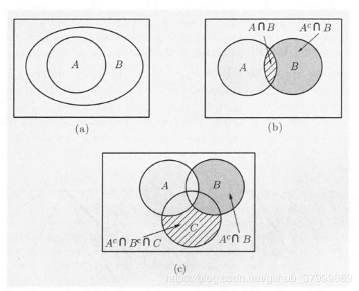
These properties, and other similar ones:

• $P(A_1\cup A_2\cup \cdots \cup A_n)\le \sum _{i=1}^{n}P(A_i)$
• $P(A_1\cup A_2\cup \cdots \cup A_n)\le P(A_1)+P(A_2\cup \cdots \cup A_n)$

1.3 条件概率（conditional probability）

Conditional probability provides us with a way to reason about the outcome of an experiment, based on partial information. In more precise terms, given an experiment, a corresponding sample space, and a probability law, suppose that we know that the outcome is within some given event $B$. We wish to quantify the likelihood that the outcome also belongs to some other given event $A$. We thus seek to construct a new probability law that takes into account the available knowledge: a probability law that for any event A. specifies the conditional probability of $A$ given $B$. denoted by $P(A|B)$.
We would like the conditional probabilities $P(A|B)$ of different events $A$ to constitute a legitimate probability law, which satisfies the probability axioms. Generalizing the argument, we introduce the following definition of conditional probability: $$P(A|B)=\frac{P(A\cap B)}{P(B)}$$In words, out of the total probability of the elements of $B$, $P(A|B)$ is the fraction that is assigned to possible outcomes that also belong to $A$.

【条件概率的概率律/性质】

• The conditional probability of an event $A$, given an event $B$ with $P(B)>0$, is defined by $$P(A|B)=\frac{P(A\cap B)}{P(B)}$$ and specifies a new (conditional) probability law on the same sample space $\Omega$. In particular, all properties of probability laws remain valid for conditional probability laws.
• Conditional probabilities can also be viewed as a probability law on a new universe $B$, because all of the conditional probability is concentrated on $B$.
• If the possible outcomes are finitely many and equally likely, then $$P(A|B)=\frac{numberofelementsofA\cap B}{numberofelementsofB}$$

【利用条件概率定义概率模型】When constructing probabilistic models for experiments that have a sequential character, it is often natural and convenient to first specify conditional probabilities and then use them to determine unconditional probabilities. The rule $P(A\cap B)=P(B)P(A|B)$, which is a restatement of the definition of conditional probability, is often helpful in this process.

【贯序树形图】We have a general rule for calculating various probabilities in conjunction with a tree-based sequential description of an experiment. In particular:

• We set up the tree so that an event of interest is associated with a leaf. We view the occurrence of the event as a sequence of steps, namely, the traversals of the branches along the path fron1 the root to the leaf.
• We record the conditional probabilities associated with the branches of the tree.
• We obtain the probability of a leaf by multiplying the probabilities recorded along the corresponding path of the tree.

In mathematical terms, we are dealing with an event $A$ which occurs if and only if each one of several events $A_1,\cdots ,A_n$ has occurred, i.e., $A=A_1\cap A_2\cap \cdot \cdot \cdot \cap A_n$. The occurrence of $A$ is viewed as an occurrence of $A_1$ , followed by the occurrence of $A_2$, then of $A_3$, etc., and it is visualized as a path with n branches, corresponding to the events $A_1,\cdots ,A_n$. The probability of $A$ is given by the following rule:

Multiplication Rule: Assuming that all of the conditioning events have positive probability, we have $$P(\bigcap _{i=1}^n{A}_i=P(A_1)P(A_2|A_1)P(A_3|A_1\cap A_2)\cdots P(A_n|\bigcap _{i=1}^{n-1}{A}_i)$$

Visualization of the multiplication rule. The intersection event
$A=A_1\cap A_2\cap \cdots \cap A_n$ is associated with a particular path on a tree that describes the experiment. We associate the branches of this path with the events $A_1\cdots A_n$. and we record next to the branches the corresponding conditional probabilities.
The final node of the path corresponds to the intersection event A, and its probability is obtained by multiplying the conditional probabilities recorded along the branches of the path

1.4 全概率定理与贝叶斯准则（total probability theorem and Bayes’ rule）

【全概率定理（Total Probability Theorem）】Let $A_1,\cdots ,A_n$ be disjoint events that form a partition of the sample space (each possible outcome is included in exactly one of the events $A_1,\cdots ,A_n$) and assume that $P(A_i)>0$, for all $i$. Then, for any event $B$, we have $$P(B)=P(A_1\cap B)+P(A_2\cap B)+\cdots +P(A_n\cap B)$$ $$=P(A_1)P(B|A_1)+\cdots +P(A_n)P(B|A_n)$$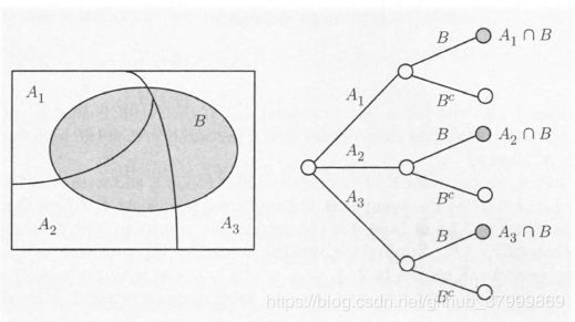
【贝叶斯准则】The total probability theorem is often used in conjunction with the following celebrated theorem, which relates conditional probabilities of the form $P(A|B)$ with conditional probabilities of the form $P(B|A)$, in which the order of the conditioning is reversed.

Let $A_1,A_2,\cdots ,A_n$ be disjoint events that form a partition of the sample space, and assume that $P(A_i)>0$, for all $i$. Then, for any event $B$ such that $P(B)>0$, we have $$P(A_i|B)=\frac{P(A_i)P(B|A_i)}{P(B)}$$ $$=\frac{P(A_i)P(B|A_i)}{P(A_1)P(B|A_1)+\cdots +P(A_n)P(B|A_n)}$$

To verify Bayes’rule. note that by the definition of conditional probability, we have $$P(A_i\cap B)=P(A_i)P(B|A_i)=P(B)P(A_i|B)$$ This yields the first equality. The second equality follows from the first by using the total probability theorem to rewrite $P(B)$.
Bayes’rule is often used for inference. There are a number of “causes” that may result in a certain “effect.” We observe the effect, and we wish to infer the cause. The events $A_1,\cdots ,A_n$ are associated with the causes and the event $B$ represents the effect. The probability $P(B|A_i)$ that the effect will be observed when the cause $A_i$ is present amounts to a probabilistic model of the cause-effect relation. Given that the effect $B$ has been observed, we wish to evaluate the probability $P(A_i|B)$ that the cause $A_i$ is present. We refer to $P(A_i|B)$ as the posterior probability of event $A_i$ given the information, to be distinguished from $P(A_i)$, which we call the prior probability

1.5 独立性

We have introduced the conditional probability $P(A|B)$ to capture the partial information that event $B$ provides about event $A$. An interesting and important special case arises when the occurrence of $B$ provides no such information and does not alter the probability that $A$ has occurred, i.e.,$$P(A|B)=P(A)$$.
When the above equality holds. we say that $A$ is independent of $B$. Note that $$P(A\cap B)=P(A)P(B)$$We adopt this latter relation as the definition of independence because it can be used even when $P(B)=0$, in which case $P(A|B)$ is undefined. The symmetry of this relation also implies that independence is a symmetric property; that is, if $A$ is independent of $B$, then $B$ is independent of $A$, and we can unambiguously say that $A$ and $B$ are independent events.
If $A$ and $B$ are independent, the occurrence of $B$ does not provide any new information on the probability of $A$ occurring. It is then intuitive that the non-occurrence of $B$ should also provide no information on the probability of $A$. Indeed. it can be verified that if $A$ and $B$ are independent, the same holds true for $A$ and $B^c$.

【条件独立】In particular, given an event C. the events A and B are called conditionally independent if $$P(A\cap B|C)=P(A|C)P(B|C)$$
To derive an alternative characterization of conditional independence, we use the definition of the conditional probability and the multiplication rule, to write $$P(A\cap B|C)=\frac{P(A\cap B\cap C)}{P(C)}$$ $$=\frac{P(C)P(B|C)P(A|B\cap C)}{P(C)}$$ $$=P(B|C)P(A|B\cap C)$$ We now compare the preceding two expressions. and after eliminating the common factor $P(B|C)$, assumed nonzero. we see that conditional independence is the same as the condition $$P(A|B\cap C)=P(A|C)$$ In words, this relation states that if $C$ is known to have occurred, the additional knowledge that $B$ also occurred does not change the probability of $A$.
【多个事件相互独立】We say that the events $A_1,A_2,\cdots ,A_n$ are independent if $$P(\bigcap _{i\in S}{A}_i)=\prod _{i\in S}P(A_i)$$ for every subset $S$ of $\{1,2,\cdots ,n\}$
【独立实验和二项概率】If an experiment involves a sequence of independent but identical stages, we say that we have a sequence of independent trials. In the special case where there are only two possible results at each stage, we say that we have a sequence of independent Bernoulli trials. The two possible results can be anything, e.g., “it rains” or “it doesn’t rain,” but we will often think in terms of coin tosses and refer to the two results as’“heads” ($H$) and "tails·’($T$).
Consider an experiment that consists of n independent tosses of a coin, in which the probability of heads is $p$, where $p$ is some number between 0 and 1. In this context, independence means that the events $A_1,A_2,\cdots ,A_n$ are independent, where $A_i$ = {$i$th toss is a head}.

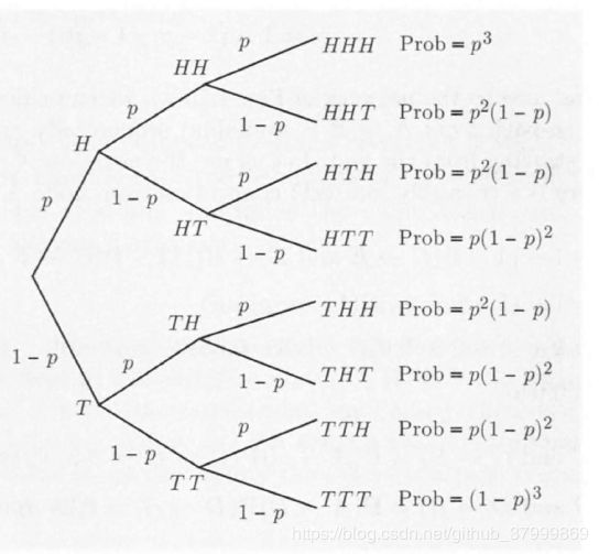
$p(k)=P(k$ heads come up in an n-toss sequence$)$,which will play an important role later. We showed above that the probability of any given sequence that contains k heads is $p^k(I-p{)}^{n-k}$, so we have $$p(k)=\left(\genfrac{}{}{0ex}{}{n}{k}\right)p^k(1-p{)}^{n-k}$$where we use the notation $$\left(\genfrac{}{}{0ex}{}{n}{k}\right)$$ means number of distinct $n$-toss sequences that contain $k$ heads.$$\left(\genfrac{}{}{0ex}{}{n}{k}\right)=\frac{n!}{k!(n-k)!}$$An alternative verification is sketched in the end-ofchapter problems. Note that the binomial probabilities $p(k)$ must add to 1, thus showing the binomial formula $$\sum _{k=0}^n\left(\genfrac{}{}{0ex}{}{n}{k}\right)p^k(1-p{)}^{n-k}=1$$