扩增子统计绘图7三元图

本网对Markdown排版支持较差，对格式不满意的用户请跳转至 或“宏基因组”公众号阅读；

写在前面

优秀的作品都有三部分曲，如骇客帝国、教父、指环王等。

扩增子系列课程也分为三部曲：

第一部《扩增子图表解读》：加速大家对同行文章的解读能力。

第二部《扩增子分析解读》：学习数据分析的基本思路和流程。

第三部《扩增子统计绘图》：即是对结果进行可视和统计检验，达到出版级的图表结果。

《扩增子统计绘图》系列文章介绍

《扩增子统计绘图》是之前发布的《扩增子图表解读》和《扩增子分析解读》的进阶篇，是在大家可以看懂文献图表，并能开展标准扩增子分析的基础上，进行结果的统计与可视化。其章节设计与《扩增子图表解读》对应，为八节课八种常用图形(箱线图、散点图、热图、曼哈顿图、火山图、维恩图、三元图和网络图)，基本满足文章常用的图片种类需求。

也适合对公司标准化分析返回结果的进一步统计、可视化及美化，达到出版级别，冲击高分文章。

本部分练习所需文件位于百度网盘，链接：http://pan.baidu.com/s/1hs1PXcw 密码：y33d。

1箱线图：Alpha多样性
2散点图：Beta多样性，PCoA, CCA
3热图：差异菌、OTU及功能
4曼哈顿图：差异OTU或Taxonomy
5火山图：差异OTU数量及变化规律
6韦恩图：比较组间共有和特有OTU或分类单元
本节需要在”3热图：差异菌、OTU及功能”和”6韦恩图”基础上继续运行

7三元图

三元图有两种用法，常用的本质上是维恩图的一种变形，但维恩图只是数字比较单调，三元图类型上是散点图，可以用点大小和颜色代表丰度、显著性等信息，来进一步丰富图片信息。而且中国的文化中有事不过三，一而再、再而三等文化；三角形成最稳定也给人稳重、信认之感，三元图的美观和实用自然必不可少。

三元图主要分两种：展示两组共有和特有显著富集OTU，展示三种特异富集OTU。详见7三元图：美的不要不要的，再多用也不过分。本文主要以绘制比较常用的两组共有和特有显著富集OTU的三角图。另一种只要分析思路清楚，大家在此基础上很容易修改出来，只是代码量是需要加倍的(6次两两比较+三次取交集)。

加载三元图的配色方案和自定义函数

# 定义常用颜色 Defined color with transparent
alpha = .7
c_yellow =          rgb(255 / 255, 255 / 255,   0 / 255, alpha)
c_blue =            rgb(  0 / 255, 000 / 255, 255 / 255, alpha)
c_orange =          rgb(255 / 255,  69 / 255,   0 / 255, alpha)
c_green =           rgb(  50/ 255, 220 / 255,  50 / 255, alpha)
c_dark_green =      rgb( 50 / 255, 200 / 255, 100 / 255, alpha)
c_very_dark_green = rgb( 50 / 255, 150 / 255, 100 / 255, alpha)
c_sea_green =       rgb( 46 / 255, 129 / 255,  90 / 255, alpha)
c_black =           rgb(  0 / 255,   0 / 255,   0 / 255, alpha)
c_grey =            rgb(180 / 255, 180 / 255,  180 / 255, alpha)
c_dark_brown =      rgb(101 / 255,  67 / 255,  33 / 255, alpha)
c_red =             rgb(200 / 255,   0 / 255,   0 / 255, alpha)
c_dark_red =        rgb(255 / 255, 130 / 255,   0 / 255, alpha)

# 三元图函数，无须理解直接调用即可 Function of ternary plot
tern_e=function (x, scale = 1, dimnames = NULL, dimnames_position = c("corner",
                                                                       "edge", "none"), dimnames_color = "black", id = NULL, id_color = "black",
                  coordinates = FALSE, grid = TRUE, grid_color = "gray", labels = c("inside",
                                                                                    "outside", "none"), labels_color = "darkgray", border = "black",
                  bg = "white", pch = 19, cex = 1, prop_size = FALSE, col = "red",
                  main = "ternary plot", newpage = TRUE, pop = TRUE, ...)
{
  labels = match.arg(labels)
  if (grid == TRUE)
    grid = "dotted"
  if (coordinates)
    id = paste("(", round(x[, 1] * scale, 1), ",", round(x[,
                                                            2] * scale, 1), ",", round(x[, 3] * scale, 1), ")",
                sep = "")
  dimnames_position = match.arg(dimnames_position)
  if (is.null(dimnames) && dimnames_position != "none")
    dimnames = colnames(x)
  if (is.logical(prop_size) && prop_size)
    prop_size = 3
  if (ncol(x) != 3)
    stop("Need a matrix with 3 columns")
  if (any(x < 0))
    stop("X must be non-negative")
  s = rowSums(x)
  if (any(s <= 0))
    stop("each row of X must have a positive sum")
  x = x/s
  top = sqrt(3)/2
  if (newpage)
    grid.newpage()
  xlim = c(-0.03, 1.03)
  ylim = c(-1, top)
  pushViewport(viewport(width = unit(1, "snpc")))
  if (!is.null(main))
    grid.text(main, y = 0.9, gp = gpar(fontsize = 18, fontstyle = 1))
  pushViewport(viewport(width = 0.8, height = 0.8, xscale = xlim,
                        yscale = ylim, name = "plot"))
  eps = 0.01
  grid.polygon(c(0, 0.5, 1), c(0, top, 0), gp = gpar(fill = bg,
                                                     col = border), ...)
  if (dimnames_position == "corner") {
    grid.text(x = c(0, 1, 0.5), y = c(-0.02, -0.02, top +
                                        0.02), label = dimnames, gp = gpar(fontsize = 12))
  }
  if (dimnames_position == "edge") {
    shift = eps * if (labels == "outside")
      8
    else 0
    grid.text(x = 0.25 - 2 * eps - shift, y = 0.5 * top +
                shift, label = dimnames[2], rot = 60, gp = gpar(col = dimnames_color))
    grid.text(x = 0.75 + 3 * eps + shift, y = 0.5 * top +
                shift, label = dimnames[1], rot = -60, gp = gpar(col = dimnames_color))
    grid.text(x = 0.5, y = -0.02 - shift, label = dimnames[3],
              gp = gpar(col = dimnames_color))
  }
  if (is.character(grid))
    for (i in 1:4 * 0.2) {
      grid.lines(c(1 - i, (1 - i)/2), c(0, 1 - i) * top,
                 gp = gpar(lty = grid, col = grid_color))
      grid.lines(c(1 - i, 1 - i + i/2), c(0, i) * top,
                 gp = gpar(lty = grid, col = grid_color))
      grid.lines(c(i/2, 1 - i + i/2), c(i, i) * top, gp = gpar(lty = grid,
                                                               col = grid_color))
      if (labels == "inside") {
        grid.text(x = (1 - i) * 3/4 - eps, y = (1 - i)/2 *
                    top, label = i * scale, gp = gpar(col = labels_color),
                  rot = 120)
        grid.text(x = 1 - i + i/4 + eps, y = i/2 * top -
                    eps, label = (1 - i) * scale, gp = gpar(col = labels_color),
                  rot = -120)
        grid.text(x = 0.5, y = i * top + eps, label = i *
                    scale, gp = gpar(col = labels_color))
      }
      if (labels == "outside") {
        grid.text(x = (1 - i)/2 - 6 * eps, y = (1 - i) *
                    top, label = (1 - i) * scale, gp = gpar(col = labels_color))
        grid.text(x = 1 - (1 - i)/2 + 3 * eps, y = (1 -
                                                      i) * top + 5 * eps, label = i * scale, rot = -120,
                  gp = gpar(col = labels_color))
        grid.text(x = i + eps, y = -0.05, label = (1 -
                                                     i) * scale, vjust = 1, rot = 120, gp = gpar(col = labels_color))
      }
    }
  xp = x[, 2] + x[, 3]/2
  yp = x[, 3] * top
  size = unit(if (prop_size)
    #emiel inserted this code. x are proportions per row.  x*s is original data matrix. s = rowsums of original data matrix (x*s)
    prop_size * rowSums(x*x*s) / max(  rowSums(x*x*s) )
    #prop_size * rowSums(    (x*s) * ((x*s)/s)) / max(  rowSums(    (x*s) * ((x*s)/s)) )
    else cex, "lines")
  grid.points(xp, yp, pch = pch, gp = gpar(col = col), default.units = "snpc",
              size = size, ...)
  if (!is.null(id))
    grid.text(x = xp, y = unit(yp - 0.015, "snpc") - 0.5 *
                size, label = as.character(id), gp = gpar(col = id_color,
                                                          cex = cex))
  if (pop)
    popViewport(2)
  else upViewport(2)
}

绘制三组比较三元图，WT对照为顶点

# merge group to mean
## 按样品名合并实验组与转置的OTU
mat_t2 = merge(sub_design[c("genotype")], t(norm), by="row.names")[,-1]
## 按实验设计求组平均值
mat_mean = aggregate(mat_t2[,-1], by=mat_t2[1], FUN=mean) # mean 
# 重新转载并去除组名
per3=t(mat_mean[,-1])
colnames(per3) = mat_mean$genotype
per3=as.data.frame(per3[rowSums(per3)>0,]) # remove all 0 OTU
#per3=per3[,tern] # reorder per3 as input
color=c(c_green,c_orange,c_red,c_grey) 

# 两底角相对于顶点显著富集的OTU，分共有和特有，类似维恩图
per3$color=color[4] # set all default # 设置点默认颜色为灰
AvC = KO_enriched
BvC = OE_enriched
C = intersect(row.names(AvC), row.names(BvC))
A = setdiff(AvC, C) 
B = setdiff(BvC, C) 
if (length(A)>0){per3[A,]$color=color[1]} 
if (length(B)>0){per3[B,]$color=color[2]} 
if (length(C)>0){per3[C,]$color=color[3]}
## output pdf and png in 8x8 inches
per3lg=log2(per3[,1:3]*100+1) # 对数变换，差OTU千分比的差距，点大小更均匀
pdf(file=paste("ter_",tern[1],tern[2],tern[3],"venn.pdf", sep=""), height = 8, width = 8)
tern_e(per3lg[,1:3], prop=T, col=per3$color, grid_color="black", labels_color="transparent", pch=19, main="Tenary Plot")
dev.off()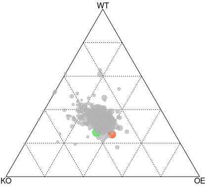

此图展示KO和OE突变体中特异或共有富集的OTU，本数据因为是测试数据，过统计显著的每组只有一个显著富集的OTU，没有共有富集的OTU。
详细的图片讲解，可参考7三元图：美的不要不要的，再多用也不过分

想了解更多宏基因组、16S文献阅读和分析相关文章，快关注“宏基因组”公众号，干货第一时间推送。

系统学习生物信息，快关注“生信宝典”，那里有几千志同道合的小伙伴一起学习。