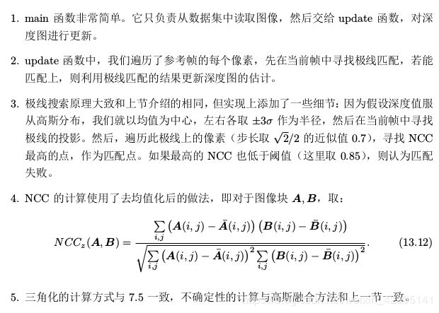
建图——单目稠密重建

目录

      • 立体视觉
      • 极线搜索与块匹配
      • 高斯分布的深度滤波器
      • 实践:

立体视觉

在稠密重建,我们需要知道每一个像素点(或大部分像素点)的距离,那么大致上有以下几种解决方案:

  1. 使用单目相机,利用移动相机之后进行三角化,测量像素的距离。
  2. 使用双目相机,利用左右目的视差计算像素的距离(多目原理相同)。
  3. 使用 RGB-D 相机直接获得像素距离。

极线搜索与块匹配

极线搜索
建图——单目稠密重建_第1张图片

  • 左边的相机观测到了某个像素 p 1 p_1 p1 。由于这是一个单目相机,无从知道它的深度,所以假设这个深度可能在某个区域之内,不妨说是某最小值到无穷远之间:(d min , +∞)。因此,该像素对应的空间点就分布在某条线段上。在另一个视角(右侧相机)看来,这条线段的投影也形成图像平面上的一条线,称为极线。当我们知道两个相机间的运动时,这条极线也是能够确定的。

  • 在特征点法中,通过特征匹配得到p2的位置,然而现在没有描述子,只能在极线上搜索和p1想的比较相似的点。(可能沿着极线一直走比较每个像素与p1的相似程度。)

块匹配

  • p 1 p_1 p1周围取一个大小为w*w的小块,然后在极线上也取很多同样大小的小块进行比较,就可以在一定程度上提高区分性。这就是所谓的块匹配(只有假设在不同图像间整个小块的灰度值不变)。
    取了 p 1 p_1 p1周围的小块,并且在极线上也取了很多个小块。不妨把p1周围的小块记成 A ∈ R w × w A ∈ R^{w×w} ARw×w,把极线上的n个小块记成 B i , i = 1... n B_i,i=1...n Bi,i=1...n。几种不同的方法计算小块与小块间的差异:
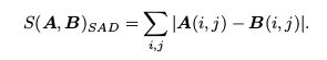
  1. SAD(Sum of Absolute Difference)。顾名思义,即取两个小块的差的绝对值之和:
    在这里插入图片描述

  2. SSD(Sum of Squared Distance)
    在这里插入图片描述

  3. NCC(Normalized Cross Correlation)(归一化互相关),计算的是两个小块的相关性:
    在这里插入图片描述

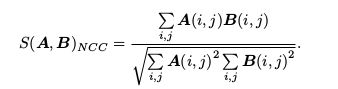
    除了这些简单的版本外,我们可以先把每个小块的均值去掉。去掉均值后,我们准许像“小块B比A整体上亮一些,但仍然很相似”这样的情况。因此比之前的更加可靠一些。

高斯分布的深度滤波器

对像素点深度的估计,本身亦可建模为一个状态估计问题,存在滤波器与非线性优化两种求解思路,采用计算量较少的滤波器方式。
下面介绍并演示高斯分布假设下的深度滤波器:

设某个像素点的深度 d 服从:
在这里插入图片描述
而每当新的数据到来,我们都会观测到它的深度。同样的,假设这次观测亦是一个高斯分布:
在这里插入图片描述
由于我们仅有观测方程而没有运动方程,所以这里深度仅用到了信息融合部分。设融合后的 d的分布为 N ( μ f u s e , σ f u s e 2 N(μ_{f use} , σ_{fuse}^2 N(μfuse,σfuse2 ),有:
在这里插入图片描述
只考虑由几何关系带来的不确定性(不考虑光度不确定性等),计算深度不确定性 σ o b s 2 σ_{obs}^2 σobs2
建图——单目稠密重建_第2张图片
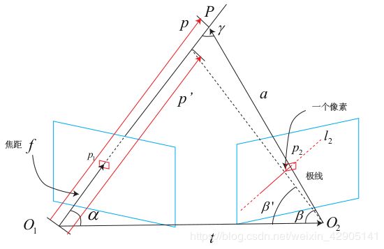
考虑某次极线搜索,我们找到了p1对应的p2点,从而观测到了p1的深度值,认为p1对应的三维点为P。
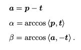
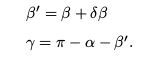
O 1 P O_1P O1P 为 p, O 1 O 2 O_1O_2 O1O2 为相机的平移 t , O 2 P O_2P O2P 记为 a。并且,把这个三角形的下面两个角记作 α, β。现在,考虑极线 l 2 l_2 l2 上存在着一个像素大小的误差,使得 β 角变成了 β ′ ,而 p 也变成了 p ′ ,并记上面那个角为 γ。我们要问的是,这一个像素的误差,会导致 p ′ 与 p 产生多大的差距呢?

由集合关系得:
在这里插入图片描述
p 2 p_2 p2 扰动一个像素,将使得 β 产生一个变化量 δβ,由于相机焦距为 f ,于是:
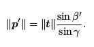
在这里插入图片描述
在这里插入图片描述
p ′ 的大小可以求得:
在这里插入图片描述
由此,我们确定了由单个像素的不确定引起的深度不确定性。如果认为极线搜索的块
匹配仅有一个像素的误差,那么就可以设:
在这里插入图片描述
如果极线搜索的不确定性大于一个像素,我们亦可按照此推导来放大这个不确定性。

估计稠密深度的一个完整的过程:

  1. 假设所有像素的深度满足某个初始的高斯分布。

  2. 当新数据产生时,通过极线搜索和块匹配确定投影点位置。

  3. 根据几何关系计算三角化后的深度及不确定性。

  4. 将当前观测融合进上一次的估计中。若收敛则停止计算,否则返回第2步。

实践:

#include 
#include 
#include 
using namespace std; 
#include 

// for sophus 
#include 
using Sophus::SE3;

// for eigen 
#include 
#include 
using namespace Eigen;

#include 
#include 
#include 

using namespace cv;

/**********************************************
* 本程序演示了单目相机在已知轨迹下的稠密深度估计
* 使用极线搜索 + NCC 匹配的方式,与书本的 13.2 节对应
* 请注意本程序并不完美,你完全可以改进它——我其实在故意暴露一些问题。
***********************************************/


// ------------------------------------------------------------------
// parameters 
const int boarder = 20; 	// 边缘宽度
const int width = 640;  	// 宽度 
const int height = 480;  	// 高度
const double fx = 481.2f;	// 相机内参
const double fy = -480.0f;
const double cx = 319.5f;
const double cy = 239.5f;
const int ncc_window_size = 2;	// NCC 取的窗口半宽度
const int ncc_area = (2*ncc_window_size+1)*(2*ncc_window_size+1); // NCC窗口面积
const double min_cov = 0.1;	// 收敛判定:最小方差
const double max_cov = 10;	// 发散判定:最大方差

// ------------------------------------------------------------------
// 重要的函数 
// 从 REMODE 数据集读取数据  
bool readDatasetFiles( 
    const string& path, 
    vector<string>& color_image_files, 
    vector<SE3>& poses 
);

// 根据新的图像更新深度估计
bool update( 
    const Mat& ref, 
    const Mat& curr, 
    const SE3& T_C_R, 
    Mat& depth, 
    Mat& depth_cov 
);

// 极线搜索 
bool epipolarSearch( 
    const Mat& ref, 
    const Mat& curr, 
    const SE3& T_C_R, 
    const Vector2d& pt_ref, 
    const double& depth_mu, 
    const double& depth_cov,
    Vector2d& pt_curr
);

// 更新深度滤波器 
bool updateDepthFilter( 
    const Vector2d& pt_ref, 
    const Vector2d& pt_curr, 
    const SE3& T_C_R, 
    Mat& depth, 
    Mat& depth_cov
);

// 计算 NCC 评分 
double NCC( const Mat& ref, const Mat& curr, const Vector2d& pt_ref, const Vector2d& pt_curr );

// 双线性灰度插值 
inline double getBilinearInterpolatedValue( const Mat& img, const Vector2d& pt ) {
    uchar* d = & img.data[ int(pt(1,0))*img.step+int(pt(0,0)) ];
    double xx = pt(0,0) - floor(pt(0,0)); 
    double yy = pt(1,0) - floor(pt(1,0));
    return  (( 1-xx ) * ( 1-yy ) * double(d[0]) +
            xx* ( 1-yy ) * double(d[1]) +
            ( 1-xx ) *yy* double(d[img.step]) +
            xx*yy*double(d[img.step+1]))/255.0;
}

// ------------------------------------------------------------------
// 一些小工具 
// 显示估计的深度图 
void plotDepth( const Mat& depth );

// 像素到相机坐标系 
inline Vector3d px2cam ( const Vector2d px ) {
    return Vector3d ( 
        (px(0,0) - cx)/fx,
        (px(1,0) - cy)/fy, 
        1
    );
}

// 相机坐标系到像素 
inline Vector2d cam2px ( const Vector3d p_cam ) {
    return Vector2d (
        p_cam(0,0)*fx/p_cam(2,0) + cx, 
        p_cam(1,0)*fy/p_cam(2,0) + cy 
    );
}

// 检测一个点是否在图像边框内
inline bool inside( const Vector2d& pt ) {
    return pt(0,0) >= boarder && pt(1,0)>=boarder 
        && pt(0,0)+boarder<width && pt(1,0)+boarder<=height;
}

// 显示极线匹配 
void showEpipolarMatch( const Mat& ref, const Mat& curr, const Vector2d& px_ref, const Vector2d& px_curr );

// 显示极线 
void showEpipolarLine( const Mat& ref, const Mat& curr, const Vector2d& px_ref, const Vector2d& px_min_curr, const Vector2d& px_max_curr );
// ------------------------------------------------------------------


int main( int argc, char** argv )
{
    if ( argc != 2 )
    {
        cout<<"Usage: dense_mapping path_to_test_dataset"<<endl;
        return -1;
    }
    
    // 从数据集读取数据
    vector<string> color_image_files; 
    vector<SE3> poses_TWC;
    bool ret = readDatasetFiles( argv[1], color_image_files, poses_TWC );
    if ( ret==false )
    {
        cout<<"Reading image files failed!"<<endl;
        return -1; 
    }
    cout<<"read total "<<color_image_files.size()<<" files."<<endl;
    
    // 第一张图
    Mat ref = imread( color_image_files[0], 0 );                // gray-scale image 
    SE3 pose_ref_TWC = poses_TWC[0];
    double init_depth   = 3.0;    // 深度初始值
    double init_cov2    = 3.0;    // 方差初始值 
    Mat depth( height, width, CV_64F, init_depth );             // 深度图
    Mat depth_cov( height, width, CV_64F, init_cov2 );          // 深度图方差 
    
    for ( int index=1; index<color_image_files.size(); index++ )
    {
        cout<<"*** loop "<<index<<" ***"<<endl;
        Mat curr = imread( color_image_files[index], 0 );       
        if (curr.data == nullptr) continue;
        SE3 pose_curr_TWC = poses_TWC[index];
        SE3 pose_T_C_R = pose_curr_TWC.inverse() * pose_ref_TWC; // 坐标转换关系: T_C_W * T_W_R = T_C_R 
        update( ref, curr, pose_T_C_R, depth, depth_cov );
        plotDepth( depth );
        imshow("image", curr);
        waitKey(1);
    }
    
    cout<<"estimation returns, saving depth map ..."<<endl;
    imwrite( "depth.png", depth );
    cout<<"done."<<endl;
    
    return 0;
}

bool readDatasetFiles(
    const string& path, 
    vector< string >& color_image_files, 
    std::vector<SE3>& poses
)
{
    ifstream fin( path+"/first_200_frames_traj_over_table_input_sequence.txt");
    if ( !fin ) return false;
    
    while ( !fin.eof() )
    {
		// 数据格式:图像文件名 tx, ty, tz, qx, qy, qz, qw ,注意是 TWC 而非 TCW
        string image; 
        fin>>image; 
        double data[7];
        for ( double& d:data ) fin>>d;
        
        color_image_files.push_back( path+string("/images/")+image );
        poses.push_back(
            SE3( Quaterniond(data[6], data[3], data[4], data[5]), 
                 Vector3d(data[0], data[1], data[2]))
        );
        if ( !fin.good() ) break;
    }
    return true;
}

// 对整个深度图进行更新
bool update(const Mat& ref, const Mat& curr, const SE3& T_C_R, Mat& depth, Mat& depth_cov )
{
#pragma omp parallel for
    for ( int x=boarder; x<width-boarder; x++ )
#pragma omp parallel for
        for ( int y=boarder; y<height-boarder; y++ )
        {
			// 遍历每个像素
            if ( depth_cov.ptr<double>(y)[x] < min_cov || depth_cov.ptr<double>(y)[x] > max_cov ) // 深度已收敛或发散
                continue;
            // 在极线上搜索 (x,y) 的匹配 
            Vector2d pt_curr; 
            bool ret = epipolarSearch ( 
                ref, 
                curr, 
                T_C_R, 
                Vector2d(x,y), 
                depth.ptr<double>(y)[x], 
                sqrt(depth_cov.ptr<double>(y)[x]),
                pt_curr
            );
            
            if ( ret == false ) // 匹配失败
                continue; 
            
			// 取消该注释以显示匹配
            showEpipolarMatch( ref, curr, Vector2d(x,y), pt_curr );
            
            // 匹配成功,更新深度图 
            updateDepthFilter( Vector2d(x,y), pt_curr, T_C_R, depth, depth_cov );
        }
}

// 极线搜索
// 方法见书 13.2 13.3 两节
bool epipolarSearch(
    const Mat& ref, const Mat& curr, 
    const SE3& T_C_R, const Vector2d& pt_ref, 
    const double& depth_mu, const double& depth_cov, 
    Vector2d& pt_curr )
{
    Vector3d f_ref = px2cam( pt_ref );
    f_ref.normalize();
    Vector3d P_ref = f_ref*depth_mu;	// 参考帧的 P 向量
    
    Vector2d px_mean_curr = cam2px( T_C_R*P_ref ); // 按深度均值投影的像素
    double d_min = depth_mu-3*depth_cov, d_max = depth_mu+3*depth_cov;
    if ( d_min<0.1 ) d_min = 0.1;
    Vector2d px_min_curr = cam2px( T_C_R*(f_ref*d_min) );	// 按最小深度投影的像素
    Vector2d px_max_curr = cam2px( T_C_R*(f_ref*d_max) );	// 按最大深度投影的像素
    
    Vector2d epipolar_line = px_max_curr - px_min_curr;	// 极线(线段形式)
    Vector2d epipolar_direction = epipolar_line;		// 极线方向 
    epipolar_direction.normalize();
    double half_length = 0.5*epipolar_line.norm();	// 极线线段的半长度
    if ( half_length>100 ) half_length = 100;   // 我们不希望搜索太多东西 
    
	// 取消此句注释以显示极线(线段)
    showEpipolarLine( ref, curr, pt_ref, px_min_curr, px_max_curr );
    
    // 在极线上搜索,以深度均值点为中心,左右各取半长度
    double best_ncc = -1.0;
    Vector2d best_px_curr; 
    for ( double l=-half_length; l<=half_length; l+=0.7 )  // l+=sqrt(2) 
    {
        Vector2d px_curr = px_mean_curr + l*epipolar_direction;  // 待匹配点
        if ( !inside(px_curr) )
            continue; 
        // 计算待匹配点与参考帧的 NCC
        double ncc = NCC( ref, curr, pt_ref, px_curr );
        if ( ncc>best_ncc )
        {
            best_ncc = ncc; 
            best_px_curr = px_curr;
        }
    }
    if ( best_ncc < 0.85f )      // 只相信 NCC 很高的匹配
        return false; 
    pt_curr = best_px_curr;
    return true;
}

double NCC (
    const Mat& ref, const Mat& curr, 
    const Vector2d& pt_ref, const Vector2d& pt_curr
)
{
    // 零均值-归一化互相关
    // 先算均值
    double mean_ref = 0, mean_curr = 0;
    vector<double> values_ref, values_curr; // 参考帧和当前帧的均值
    for ( int x=-ncc_window_size; x<=ncc_window_size; x++ )
        for ( int y=-ncc_window_size; y<=ncc_window_size; y++ )
        {
            double value_ref = double(ref.ptr<uchar>( int(y+pt_ref(1,0)) )[ int(x+pt_ref(0,0)) ])/255.0;
            mean_ref += value_ref;
            
            double value_curr = getBilinearInterpolatedValue( curr, pt_curr+Vector2d(x,y) );
            mean_curr += value_curr;
            
            values_ref.push_back(value_ref);
            values_curr.push_back(value_curr);
        }
        
    mean_ref /= ncc_area;
    mean_curr /= ncc_area;
    
	// 计算 Zero mean NCC
    double numerator = 0, demoniator1 = 0, demoniator2 = 0;
    for ( int i=0; i<values_ref.size(); i++ )
    {
        double n = (values_ref[i]-mean_ref) * (values_curr[i]-mean_curr);
        numerator += n;
        demoniator1 += (values_ref[i]-mean_ref)*(values_ref[i]-mean_ref);
        demoniator2 += (values_curr[i]-mean_curr)*(values_curr[i]-mean_curr);
    }
    return numerator / sqrt( demoniator1*demoniator2+1e-10 );   // 防止分母出现零
}

bool updateDepthFilter(
    const Vector2d& pt_ref, 
    const Vector2d& pt_curr, 
    const SE3& T_C_R,
    Mat& depth, 
    Mat& depth_cov
)
{
    // 我是一只喵
    // 不知道这段还有没有人看
    // 用三角化计算深度
    SE3 T_R_C = T_C_R.inverse();
    Vector3d f_ref = px2cam( pt_ref );
    f_ref.normalize();
    Vector3d f_curr = px2cam( pt_curr );
    f_curr.normalize();
    
    // 方程
    // d_ref * f_ref = d_cur * ( R_RC * f_cur ) + t_RC
    // => [ f_ref^T f_ref, -f_ref^T f_cur ] [d_ref] = [f_ref^T t]
    //    [ f_cur^T f_ref, -f_cur^T f_cur ] [d_cur] = [f_cur^T t]
    // 二阶方程用克莱默法则求解并解之
    Vector3d t = T_R_C.translation();
    Vector3d f2 = T_R_C.rotation_matrix() * f_curr; 
    Vector2d b = Vector2d ( t.dot ( f_ref ), t.dot ( f2 ) );
    double A[4];
    A[0] = f_ref.dot ( f_ref );
    A[2] = f_ref.dot ( f2 );
    A[1] = -A[2];
    A[3] = - f2.dot ( f2 );
    double d = A[0]*A[3]-A[1]*A[2];
    Vector2d lambdavec = 
        Vector2d (  A[3] * b ( 0,0 ) - A[1] * b ( 1,0 ),
                    -A[2] * b ( 0,0 ) + A[0] * b ( 1,0 )) /d;
    Vector3d xm = lambdavec ( 0,0 ) * f_ref;
    Vector3d xn = t + lambdavec ( 1,0 ) * f2;
    Vector3d d_esti = ( xm+xn ) / 2.0;  // 三角化算得的深度向量
    double depth_estimation = d_esti.norm();   // 深度值
    
    // 计算不确定性(以一个像素为误差)
    Vector3d p = f_ref*depth_estimation;
    Vector3d a = p - t; 
    double t_norm = t.norm();
    double a_norm = a.norm();
    double alpha = acos( f_ref.dot(t)/t_norm );
    double beta = acos( -a.dot(t)/(a_norm*t_norm));
    double beta_prime = beta + atan(1/fx);
    double gamma = M_PI - alpha - beta_prime;
    double p_prime = t_norm * sin(beta_prime) / sin(gamma);
    double d_cov = p_prime - depth_estimation; 
    double d_cov2 = d_cov*d_cov;
    
    // 高斯融合
    double mu = depth.ptr<double>( int(pt_ref(1,0)) )[ int(pt_ref(0,0)) ];
    double sigma2 = depth_cov.ptr<double>( int(pt_ref(1,0)) )[ int(pt_ref(0,0)) ];
    
    double mu_fuse = (d_cov2*mu+sigma2*depth_estimation) / ( sigma2+d_cov2);
    double sigma_fuse2 = ( sigma2 * d_cov2 ) / ( sigma2 + d_cov2 );
    
    depth.ptr<double>( int(pt_ref(1,0)) )[ int(pt_ref(0,0)) ] = mu_fuse; 
    depth_cov.ptr<double>( int(pt_ref(1,0)) )[ int(pt_ref(0,0)) ] = sigma_fuse2;
    
    return true;
}

// 后面这些太简单我就不注释了(其实是因为懒)
void plotDepth(const Mat& depth)
{
    imshow( "depth", depth*0.4 );
    waitKey(1);
}

void showEpipolarMatch(const Mat& ref, const Mat& curr, const Vector2d& px_ref, const Vector2d& px_curr)
{
    Mat ref_show, curr_show;
    cv::cvtColor( ref, ref_show, CV_GRAY2BGR );
    cv::cvtColor( curr, curr_show, CV_GRAY2BGR );
    
    cv::circle( ref_show, cv::Point2f(px_ref(0,0), px_ref(1,0)), 5, cv::Scalar(0,0,250), 2);
    cv::circle( curr_show, cv::Point2f(px_curr(0,0), px_curr(1,0)), 5, cv::Scalar(0,0,250), 2);
    
    imshow("ref", ref_show );
    imshow("curr", curr_show );
    waitKey(1);
}

void showEpipolarLine(const Mat& ref, const Mat& curr, const Vector2d& px_ref, const Vector2d& px_min_curr, const Vector2d& px_max_curr)
{

    Mat ref_show, curr_show;
    cv::cvtColor( ref, ref_show, CV_GRAY2BGR );
    cv::cvtColor( curr, curr_show, CV_GRAY2BGR );
    
    cv::circle( ref_show, cv::Point2f(px_ref(0,0), px_ref(1,0)), 5, cv::Scalar(0,255,0), 2);
    cv::circle( curr_show, cv::Point2f(px_min_curr(0,0), px_min_curr(1,0)), 5, cv::Scalar(0,255,0), 2);
    cv::circle( curr_show, cv::Point2f(px_max_curr(0,0), px_max_curr(1,0)), 5, cv::Scalar(0,255,0), 2);
    cv::line( curr_show, Point2f(px_min_curr(0,0), px_min_curr(1,0)), Point2f(px_max_curr(0,0), px_max_curr(1,0)), Scalar(0,255,0), 1);
    
    imshow("ref", ref_show );
    imshow("curr", curr_show );
    waitKey(1);
}

注解:

建图——单目稠密重建_第3张图片

你可能感兴趣的:(SLAM,#,VSLAM)