吴恩达Coursera深度学习课程 deeplearning.ai (4-4) 神经风格转换--编程作业

吴恩达Coursera深度学习课程 deeplearning.ai (4-4) 神经风格转换–编程作业

注：由于这个作业目前未找到完整的中文版的，所以楼主综合了几篇不完整的，自己完整运行了一遍（python3.5.4），整理了一下。第一次写博客，有问题大家一起讨论，谢谢。

资料下载：
链接：https://pan.baidu.com/s/1wKgjZ6E7cnkiyc6e5EU-zQ
提取码：baue
program.py为完整的神经风格转移程序代码。

在这次作业中，你将:
实现神经风格的传递算法；
使用你的算法生成新的艺术图像；
你学习过的大多数算法都是通过优化成本函数来获得一组参数值。在本次学习中，你将通过优化成本函数得到像素值!
导入需要的包：

import os
import sys
import scipy.io
import scipy.misc
import matplotlib.pyplot as plt
from matplotlib.pyplot import imshow
from PIL import Image
from nst_utils import *
import numpy as np
import tensorflow as tf
#matplotlib inline

**

1.问题描述

**
神经风格转移(NST)是深度学习中最有趣的技术之一。如下图所示，它融合了两个图像，即一个“内容”图像©和一个“风格”图像(S)，以创建一个“生成”图像(G)。生成的图像G将图像C的“内容”与图像S的“风格”相结合。
在本例中，你将生成一幅卢浮宫图片与领导印象派运动的克劳德·莫奈的画（风格图像S）混合起来的图片。如下所示：

**

2.迁移学习

**
神经风格转换(NST)使用之前训练过的卷积网络，并在此基础上进行构建。使用针对不同任务训练的网络并将其应用于新任务的思想称为迁移学习。
在最初的NST论文(https:/larxiv.org/abs/1508.06576)之后，我们将使用VGG网络。具体来说，我们将使用VGG-19, VGG网络的19层版本。这个模型已经在非常大的ImageNet数据库上进行了训练，因此学会了识别各种低级别特征(在较浅的层)和高级别特征(在较深的层)。
运行以下代码从VGG模型加载参数。这可能需要几秒钟。
**

model = load_vgg_model("pretrained-model/imagenet-vgg-verydeep-19.mat")
print(model)

结果：

{'conv4_1': , 'conv5_2': , 'avgpool5': , 'conv4_3': , 'conv5_1': , 'avgpool2': , 'conv1_1': , 'input': , 'avgpool1': , 'avgpool3': , 'conv2_1': , 'avgpool4': , 'conv3_1': , 'conv1_2': , 'conv5_3': , 'conv3_4': , 'conv5_4': , 'conv4_4': , 'conv3_2': , 'conv2_2': , 'conv3_3': , 'conv4_2': }

**
该模型存储在python字典中，其中每个变量名都是关键字，对应的值是一个包含该变量值的张量。要通过这个网络运行图像，您只需将图像提供给模型。在TensorFlow中，你可以使用下面的tf.assign：

model["input"].assign(image)

**
这将图像指定为模型的输入。在此之后，如果你想访问某个特定层的激活，例如第4_2层。当网络在该图像上运行时,我们可以在conv4_2上运行一个tensor session，如下所示：

sess.run(model["conv4_2"])

3.神经风格转换

我们将分三步构建NST算法:
（1）构建内容成本函数 J（C,G)
（2）构建风格成本函数
（3)计算总的成本函数

3.1 计算内容成本函数（content function）
**
在本文的例子中，选取卢浮宫louvre_small.ipg图片作为内容图片。

content_image = scipy.misc.imread("images/louvre_small.jpg")
imshow(content_image)
plt.show()

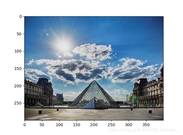
在内容图中，卢浮宫的金字塔被巴黎的古建筑包围着，在晴朗的天空下有几朵白云。

3.1.1如何确保生成图像（G）与内容图像（C）匹配
**
正如我们在课堂上看到的，卷积神经网络较早的(较浅的)层倾向于检测较低层次的特征，如边缘和简单的纹理，较晚的(较深的)层倾向于检测较高层次的特征，如更复杂的纹理和对象类。
我们希望“生成”的图像G具有与输入图像c类似的内容。假设您选择了某个层的激活来表示图像的内容。在实践中，如果您选择了网络中间的一个层——既不太浅也不太深——您将获得最令人赏心悦目的结果。(当你完成这个练习后，可以自由地回来尝试使用不同的图层，看看结果是如何变化的。)
假设你选择了一个特殊的隐藏层。现在，将图像C设置为预先训练好的VGG网络的输入，并运行正向传播。a^（C） 为你选择的层中的隐藏层激活。(在课堂上，我们把它写成了a^（C）。但是这里我们要去掉上标[l]来简化符号)这是$n_H\times n_W\times n_C$的张量。对图像G重复这个过程:将G设置为输入，然后进行前向传播。使a^（G） 为对应的隐含层激活。我们将把内容成本函数定义为:
$$J_{content}(C,G)=\frac{1}{4\times (n_H\times n_W\times n_C)}\sum (a^{(}C)-a^{(}G）{)}^2$$
这里，$n_H$、$n_W$和$n_C$是你选择的隐含层的高度、宽度和通道数，在成本中以归一项出现。为清晰起见，请注意a^（C）和a^（G）是对应于隐藏层激活的卷。为了计算成本$J_{content}(C,G)$,将这些三维卷积展开成一个二维矩阵可以便于计算,如下所示(技术上这个展开的步骤不需要计算$J_{content}(C,G)$,但这将是良好的实践,当你以后需要执行类似的操作计算$J_{style}(C,G)$时。

练习：使用tensorflow计算内容成本
说明:实现该功能的3个步骤是:
1.从a_G中获取维度:
要从张量X中检索维度，可以使用:X.get_shape().as_list()
2.如上图一样展开一个a_C和a_G
如果你遇到了问题，看看：https://www.tensorflow.org/versions/r1.3/api_docs/python/tf/transpose和https://www.tensorflow.org/versions/r1.2/api_docs/python/tf/reshape
3.计算内容成本：
如果你遇到了问题，看看：
https://www.tensorflow.org/api_docs/python/tf/reduce_sum
https://www.tensorflow.org/api_docs/python/tf/square
https://www.tensorflow.org/api_docs/python/tf/subtract

# GRADED FUNCTION: compute_content_cost

def compute_content_cost(a_C, a_G):
    """
    Computes the content cost
    
    Arguments:
    a_C -- tensor of dimension (1, n_H, n_W, n_C), hidden layer activations representing content of the image C 
    a_G -- tensor of dimension (1, n_H, n_W, n_C), hidden layer activations representing content of the image G
    
    Returns: 
    J_content -- scalar that you compute using equation 1 above.
    """
    
    ### START CODE HERE ###
    # Retrieve dimensions from a_G (≈1 line)
    m, n_H, n_W, n_C = a_G.get_shape().as_list()
    
    # Reshape a_C and a_G (≈2 lines)
    a_C_unrolled = tf.reshape(a_C,(n_H * n_W,n_C))
    a_G_unrolled = tf.reshape(a_G,(n_H * n_W,n_C))
    
    # compute the cost with tensorflow (≈1 line)
    J_content = 1/(4*n_H*n_W*n_C) * tf.reduce_sum(tf.square(tf.subtract(a_C_unrolled , a_G_unrolled)))
    ### END CODE HERE ###
    
    return J_content

tf.reset_default_graph() 

with tf.Session() as test:
    tf.set_random_seed(1)
    a_C = tf.random_normal([1, 4, 4, 3], mean=1, stddev=4)
    a_G = tf.random_normal([1, 4, 4, 3], mean=1, stddev=4)
    J_content = compute_content_cost(a_C, a_G)
    print("J_content = " + str(J_content.eval()))

执行结果：J_content = 6.7655935

期望的输出结果：J_content = 6.76559
*
内容成本采用神经网络的隐含层激活，并测量a^（C） 和a^（G） 的差异。
当我们稍后最小化内容成本时，这将有助于确保G具有与C类似的内容。

3.2计算风格成本
对于我们的运行示例，我们将使用以下风格图像:

style_image = scipy.misc.imread("images/monet.jpg")
imshow(style_image)
plt.show()

执行结果：

这幅画是印象派风格的。
让我们看看如何定义一个“风格”成本函数。

3.2.1风格矩阵
风格矩阵又叫格拉姆矩阵(Gram matrix)。在线性代数中格拉姆矩阵G由一组向量$(v_1,\dots ,v_n)$相互点乘(对应元素相乘)得到
$$G_{ij}=v_i^T{v}^j=np.dot(v^i,v^j)$$
换言之，$G_{ij}$比较了$v^i$和$v^j$之间的相似度：如果它们高度相似，你会期望它们有一个大的点积，因此$G_{ij}$会很大。
注意，这里使用的变量名有一个冲突。我们使用的是文献中常用的术语，但是G用于表示风格矩阵(Gram矩阵)和生成的图像G。我们将尝试确保我们所引用的G总是在上下文中明确的。
在NST中，你可以通过将“展开的”矩阵与它们的转置矩阵相乘来计算风格矩阵:

结果是一个$(n_c,n_c)$维矩阵，其中$n_c)$是卷积核的数量。$G_{ij}$值是filiter i的激活与filter j的激活之间的相似性。
Gram矩阵的一个重要部分是，对角线元素(如$G_{ii}$)也可以度量filter i的活跃度。例如，假设filter i正在检测图像中的垂直纹理。然后$G_{ii}$测量垂直纹理在整个图像中的普遍程度:如果$G_{ii}$很大，这意味着图像有很多垂直纹理。
通过捕捉不同类型特征的普遍程度($G_{ii}$)以及不同特征同时出现的程度($G_{ij}$)，风格矩阵G可以衡量图像的样式。
练习:使用TensorFlow计算矩阵A的Gram矩阵，公式为:A的Gram矩阵为$G_A=A{A}^T$。如果你遇到了问题，看看
https://www.tensorflow.org/api_docs/python/tf/matmul
https://www.tensorflow.org/api_docs/python/tf/transpose

def gram_matrix(A):
    """
    Argument:
    A -- matrix of shape (n_C, n_H*n_W)

    Returns:
    GA -- Gram matrix of A, of shape (n_C, n_C)
    """

    ### START CODE HERE ### (≈1 line)
    GA = tf.matmul(A,tf.transpose(A))
    ### END CODE HERE ###

    return GA

tf.reset_default_graph()

with tf.Session() as test:
    tf.set_random_seed(1)
    A = tf.random_normal([3, 2*1], mean=1, stddev=4)
    GA = gram_matrix(A)

    print("GA = " + str(GA.eval()))

**
执行结果：

GA = [[ 6.422305 -4.429122 -2.096682]
 [-4.429122 19.465837 19.563871]
 [-2.096682 19.563871 20.686462]]

3.2.2 风格成本
生成风格矩阵(格拉姆矩阵)后,你的目标是最小化的“风格”图像S和“生成”图像G的格拉姆矩阵之间的距离 。现在,我们只使用一个隐藏层$a^{[l]}$,这一层相应的风格成本定义为:
$$J_{style}(C,G)=\frac{1}{4\times ((n_C{)}^2\times (n_H\times n_W{)}^2)}\sum (G^{(S)}-G^{(G）}{)}^2$$
其中$G^{(S)}$和$G^{(G)}$分别为“风格”图像和“生成”图像的Gram矩阵，利用网络中特定隐含层的隐含层激活值计算得到。

练习:计算单层的风格成本。
说明:实现该功能的3个步骤是:
1.从隐藏层获取激活值维度a_G:
要从张量X中获得维度，可以使用: X.get_shape().as_list()
2.将隐藏层激活值a_S和a_G展开到二维矩阵中，如上图所示。
可以点击下面查看：
https://www.tensorflow.org/versions/r1.3/api_docs/python/tf/transpose
https://www.tensorflow.org/versions/r1.2/api_docs/python/tf/reshape
3.计算S和G的风格矩阵（运用前面的函数）。
4.计算风格成本。

# GRADED FUNCTION: compute_layer_style_cost

def compute_layer_style_cost(a_S, a_G):
    """
    Arguments:
    a_S -- tensor of dimension (1, n_H, n_W, n_C), hidden layer activations representing style of the image S 
    a_G -- tensor of dimension (1, n_H, n_W, n_C), hidden layer activations representing style of the image G
    
    Returns: 
    J_style_layer -- tensor representing a scalar value, style cost defined above by equation (2)
    """
    
    ### START CODE HERE ###
    # Retrieve dimensions from a_G (≈1 line)
    m, n_H, n_W, n_C = a_G.get_shape().as_list()
    
    # Reshape the images to have them of shape (n_C, n_H*n_W) (≈2 lines)
    a_S = tf.reshape(a_S,(n_H*n_W,n_C))
    a_G = tf.reshape(a_G,(n_H*n_W,n_C))

    # Computing gram_matrices for both images S and G (≈2 lines)
    GS = gram_matrix(tf.transpose(a_S))
    GG = gram_matrix(tf.transpose(a_G))
    
    # Computing the loss (≈1 line)
    J_style_layer =1/(4 * (n_C **2) * ((n_H * n_W) **2)) * tf.reduce_sum(tf.square(tf.subtract(GS,GG))) 
    
    ### END CODE HERE ###
    
    return J_style_layer

tf.reset_default_graph()

with tf.Session() as test:
    tf.set_random_seed(1)
    a_S = tf.random_normal([1, 4, 4, 3], mean=1, stddev=4)
    a_G = tf.random_normal([1, 4, 4, 3], mean=1, stddev=4)
    J_style_layer = compute_layer_style_cost(a_S, a_G)
    
    print("J_style_layer = " + str(J_style_layer.eval()))

执行结果：

J_style_layer = 9.190278

3.2.3风格权重
到目前为止，你获得了一层的风格。如果我们从几个不同的层“合并”样式成本，我们会得到更好的结果。在完成这个练习之后，你可以自由地回来尝试不同的权重，看看它如何改变生成的图像G。这是一个相当合理的默认值:

STYLE_LAYERS = [
    ('conv1_1', 0.2),
    ('conv2_1', 0.2),
    ('conv3_1', 0.2),
    ('conv4_1', 0.2),
    ('conv5_1', 0.2)]

你可以合并不同层的风格成本，如下所示：
$$J_{style}(S,G)=\sum _l{\lambda }^{[l]}{J}_{style}^{[l]}(S,G)$$
${\lambda }^{[l]}$的值在STYLE_LAYERS中给出了.
我们实现了compute_style_cost(…)函数。它只是简单地调用你的compute_layer_style_cost(…)几次。并使用STYLE_LAYERS中的值对结果进行加权。通读一遍，确保你理解了它在做什么.

def compute_style_cost(model, STYLE_LAYERS):
    """
    Computes the overall style cost from several chosen layers
    
    Arguments:
    model -- our tensorflow model
    STYLE_LAYERS -- A python list containing:
                        - the names of the layers we would like to extract style from
                        - a coefficient for each of them
    
    Returns: 
    J_style -- tensor representing a scalar value, style cost defined above by equation (2)
    """
    
    # initialize the overall style cost
    J_style = 0

    for layer_name, coeff in STYLE_LAYERS:

        # Select the output tensor of the currently selected layer
        out = model[layer_name]

        # Set a_S to be the hidden layer activation from the layer we have selected, by running the session on out
        a_S = sess.run(out)

        # Set a_G to be the hidden layer activation from same layer. Here, a_G references model[layer_name] 
        # and isn't evaluated yet. Later in the code, we'll assign the image G as the model input, so that
        # when we run the session, this will be the activations drawn from the appropriate layer, with G as input.
        a_G = out
        
        # Compute style_cost for the current layer
        J_style_layer = compute_layer_style_cost(a_S, a_G)

        # Add coeff * J_style_layer of this layer to overall style cost
        J_style += coeff * J_style_layer

    return J_style

注意:在上面for-loop的inner-loop中，a_G是一个张量，还没有被求值。当我们在下面的model_nn()中运行TensorFlow graph时，它将在每次迭代中进行评估和更新。
图像的风格可以使用隐层激活的Gram矩阵来表示。然而，我们通过结合多层的激活值得到了更好的结果。这与内容表示不同，内容表示通常只使用一个隐藏层就足够了。
最小化风格成本将导致图像G符合图像S的风格。

3.3确定要优化的总成本
最后，让我们创建一个使风格和内容成本最小化的成本函数。这个公式是:
$$J(G)=\alpha J_{content}(C,G)+\beta J_{style}(C,G)$$
练习:实现总成本函数，其中包括内容成本和风格成本。

# GRADED FUNCTION: total_cost

def total_cost(J_content, J_style, alpha = 10, beta = 40):
    """
    Computes the total cost function
    
    Arguments:
    J_content -- content cost coded above
    J_style -- style cost coded above
    alpha -- hyperparameter weighting the importance of the content cost
    beta -- hyperparameter weighting the importance of the style cost
    
    Returns:
    J -- total cost as defined by the formula above.
    """
    
    ### START CODE HERE ### (≈1 line)
    J = alpha * J_content + beta * J_style
    ### END CODE HERE ###
    
    return J

tf.reset_default_graph()

with tf.Session() as test:
    np.random.seed(3)
    J_content = np.random.randn()    
    J_style = np.random.randn()
    J = total_cost(J_content, J_style)
    print("J = " + str(J))

执行结果：J = 35.34667875478276

总成本是内容成本$J_{content}(C,G)$和风格成本$J_{style}(C,G)$的线性组合。
$\alpha$和$\beta$是调节内容和风格之间的相对权重的超参数。

4.求解最优化问题
最后，让我们把所有的东西放在一起来实现神经风格转换!以下是这个项目将要做的事情:
1. 创建一个Interactive Session
2. 加载内容图像
3. 加载样式图像
4. 随机初始化要生成的图像
5. 加载VGG16模型
6. 建立TensorFlow graph：
通过VGG16模型运行内容图像并计算内容成本；
通过VGG16模型运行风格图像并计算风格成本；
计算总成本；
定义优化器和学习率。
7. 初始化TensorFlow graph并在大量迭代中运行它，在每一次迭代中更新生成的图像。
让我们详细地过一遍每个步骤。
你已经实现了总成本J(G)。现在我们将使用TensorFlow来对G进行优化。要做到这一点，你的程序必须重置graph并使用“Interactive Session”。与常规session不同，“Interactive Session”将自己安装为构建graph的默认session。这允许你运行变量，而不需要经常引用session对象，这简化了代码。
让我们开始Interactive Session吧。

# Reset the graph
tf.reset_default_graph()

# Start interactive session
sess = tf.InteractiveSession()

让我们对“内容”图像(卢浮宫的图片)加载、整形和归一化操作:

content_image = scipy.misc.imread("images/louvre_small.jpg")
content_image = reshape_and_normalize_image(content_image)

让我们对“风格”图像(莫奈的画)加载、整形和归一化操作:

style_image = scipy.misc.imread("images/monet.jpg")
style_image = reshape_and_normalize_image(style_image)

现在，我们将“生成的”图像初始化为从内容图像创建的带噪声图像。通过初始化生成的图像的像素，使其主要是噪声，但仍然与内容图像有轻微的相关性，这将有助于“生成”图像的内容更快地匹配“内容”图像的内容。(可以在nst_utils.py中查看generate_noise_image(…))

generated_image = generate_noise_image(content_image)
#imshow(generated_image[0])

接下来，如第(2)部分所述，让我们加载VGG16模型。

model = load_vgg_model("pretrained-model/imagenet-vgg-verydeep-19.mat")

为了让程序计算内容成本，我们现在将分配一个a_C和一个a_G作为适当的隐含层激活。我们将使用conv4_2层来计算内容成本。下面的代码做了以下工作:
1. 将内容图像指定为VGG模型的输入。
2. 设a_C作为“conv4_2”层的隐含层激活的张量。
3. 设a_G作为同一层的隐含层激活的张量。
4. 使用a_C和a_G计算内容成本。

# Assign the content image to be the input of the VGG model.  
sess.run(model['input'].assign(content_image))

# Select the output tensor of layer conv4_2
out = model['conv4_2']

# Set a_C to be the hidden layer activation from the layer we have selected
a_C = sess.run(out)

# Set a_G to be the hidden layer activation from same layer. Here, a_G references model['conv4_2'] 
# and isn't evaluated yet. Later in the code, we'll assign the image G as the model input, so that
# when we run the session, this will be the activations drawn from the appropriate layer, with G as input.
a_G = out

# Compute the content cost
J_content = compute_content_cost(a_C, a_G)

注意:在这里，a_C是一个张量，还没有被赋值。当我们在下面的model_nn()中运行Tensorflow graph时，它将在每次迭代中被评价和更新。

    
# Assign the input of the model to be the "style" image 
sess.run(model['input'].assign(style_image))

# Compute the style cost
J_style = compute_style_cost(model, STYLE_LAYERS)

练习:现在已经有了$J_{content}$和$J_{style}$，通过调用total_cost()计算总成本J。用alpha = 10和beta = 40。

### START CODE HERE ### (1 line)
J = total_cost(J_content,J_style,10,40)
### END CODE HERE ###

你之前已经学习了如何在TensorFlow中设置Adam优化器。让我们在这里这样做，使用2.0的学习率。见参考
https://www.tensorflow.org/api_docs/python/tf/train/AdamOptimizer

# define optimizer (1 line)
optimizer = tf.train.AdamOptimizer(2.0)

# define train_step (1 line)
train_step = optimizer.minimize(J)

练习:实现model_nn()函数，该函数初始化tensorflow graph的变量，将输入图像(初始生成的图像)指定为VGG16模型的输入，并多次运行train_step。

def model_nn(sess, input_image, num_iterations = 200):
    
    # Initialize global variables (you need to run the session on the initializer)
    ### START CODE HERE ### (1 line)
    sess.run(tf.global_variables_initializer())
    ### END CODE HERE ###
    
    # Run the noisy input image (initial generated image) through the model. Use assign().
    ### START CODE HERE ### (1 line)
    generated_image = sess.run(model["input"].assign(input_image))
    ### END CODE HERE ###
    
    for i in range(num_iterations):
    
        # Run the session on the train_step to minimize the total cost
        ### START CODE HERE ### (1 line)
        sess.run(train_step)
        ### END CODE HERE ###
        
        # Compute the generated image by running the session on the current model['input']
        ### START CODE HERE ### (1 line)
        generated_image = sess.run(model["input"])
        ### END CODE HERE ###

        # Print every 20 iteration.
        if i%20 == 0:
            Jt, Jc, Js = sess.run([J, J_content, J_style])
            print("Iteration " + str(i) + " :")
            print("total cost = " + str(Jt))
            print("content cost = " + str(Jc))
            print("style cost = " + str(Js))
            
            # save current generated image in the "/output" directory
            save_image("output/" + str(i) + ".png", generated_image)
    
    # save last generated image
    save_image('output/generated_image.jpg', generated_image)
    
    return generated_image

运行以下程序生成一个艺术图像。在CPU上运行，每20次迭代大约需要2分钟的时间。但是在140次迭代之后，你就可以开始观察有吸引力的结果了。神经风格转移通常使用gpu进行训练。

model_nn(sess, generated_image)

执行结果：

Iteration 0 :
total cost = 4936883000.0
content cost = 7881.8374
style cost = 123420110.0
Iteration 20 :
total cost = 931767230.0
content cost = 15151.004
style cost = 23290394.0
Iteration 40 :
total cost = 477016350.0
content cost = 16802.11
style cost = 11921208.0
Iteration 60 :
total cost = 306887400.0
content cost = 17393.8
style cost = 7667836.0
Iteration 80 :
total cost = 224284830.0
content cost = 17652.46
style cost = 5602707.5
Iteration 100 :
total cost = 177648640.0
content cost = 17878.877
style cost = 4436746.5
Iteration 120 :
total cost = 147074480.0
content cost = 18052.498
style cost = 3672348.8
Iteration 140 :
total cost = 125348056.0
content cost = 18212.635
style cost = 3129148.2
Iteration 160 :
total cost = 108879560.0
content cost = 18354.621
style cost = 2717400.5
Iteration 180 :
total cost = 95958260.0
content cost = 18494.342
style cost = 2394332.8

程序运行完以后，可以在output文件夹中看到生成的图像。

5.用自己的图像进行测试
1.将自己的图片调为（400*300）的大小；
2.将图片存入images文件夹中；
3.修改3.4节中的代码：

content_image = scipy.misc.imread("images/my_content.jpg")
style_image = scipy.misc.imread("images/my_style.jpg")

4.重新运行程序

参考资料：
（1）https://github.com/Wasim37/deeplearning-assignment/blob/master/4%20卷积神经网络/Week4%20特殊的应用/Neural%20Style%20Transfer/Art%20Generation%20with%20Neural%20Style%20Transfer-v2-answer.ipynb
（2）https://blog.csdn.net/haoyutiangang/article/details/81125659
（3）https://blog.csdn.net/u013733326/article/details/80767079