fbprophet案例之python实现

目的

     上一篇博文翻译了fbprophet所参考的文献，本篇内容将给出模拟的时间序列，验证下fbpropeht的精度，以及尝试下如何调参；

1.正弦波和矩形波叠加

1.1 数据生成过程

     生成一个频率为15分钟的时间序列，其中每一天的数据是一个正弦波，如果是周末，则需要在正弦波上加1，非周末加0，即正弦波的周期是96，矩形波的周期是$96\cdot 7$，假设生成100天的数据，数据起点为2013-01-01，其中2013-04-04以及之后的数据作为样本外检验样本；
$$y(t)=sin(\frac{2\pi t}{96})+1_t(t\in 周末)$$

1.2 数据模拟的python代码

#!/usr/bin/env python
# coding: utf-8

import logging
import numpy as np
import pandas as pd
from fbprophet import Prophet
from matplotlib import pyplot as plt
import matplotlib.pyplot as plt
from fbprophet.diagnostics import cross_validation
logging.getLogger('fbprophet').setLevel(logging.ERROR)
import warnings


warnings.filterwarnings("ignore")
"""prophet的所有periods都默认为最小1天为单位
"""
d = 100*2*np.pi/(96*100-1)
y0 = np.sin(np.arange(0, 100*2*np.pi+d, d))
dates = pd.date_range(start='20130101', periods=len(y0), freq="15min")
tmp = np.zeros([len(y0)])
tmp[dates.weekday==0] = 1
tmp[dates.weekday==6] = 1
y = tmp + 1*y0

df = pd.DataFrame(y[0:len(dates)], index=dates).reset_index()
df.rename(columns={0:"y", "index":"ds"}, inplace=True)
df_train=df[df.ds<'2013-04-04']
df_test = df[df.ds>='2013-04-04']

plt.figure(1,figsize=(12,8))
plt.subplot(221)
plt.plot(df[0:96*14]["ds"], tmp[0:96*14], 'b--')
plt.xticks(rotation=45)
plt.subplot(222)
plt.plot(df[0:96*14]["ds"], y0[0:96*14], 'r--')
plt.xticks(rotation=45)
plt.subplot(212)
plt.plot(df[0:96*14]["ds"], df[0:96*14]["y"])
plt.xticks(rotation=45)
plt.show()

1.3 propeht模型拟合

     由于知道数据中含有两个周期，即以96（1天）和96·7（7天）为周期，那么编写prophet的模型也比较简单，代码如下：

m = Prophet(growth="linear", n_changepoints=0,
            yearly_seasonality=False,
            weekly_seasonality=False,
            daily_seasonality=False)

# 设置傅里叶级数的展开项数为5，后期我们会发现，这个参数太小，不足以用正余弦波来表示一个矩形波
m.add_seasonality(name='b', period=1, fourier_order=5)
m.add_seasonality(name='weekly', period=7, fourier_order=20)
m.fit(df_train)
# 由于是15分钟频率的数据，因此不能用propeht自带的make_future_dataframe函数，
# 这个函数只支持生成日度数据的时间标签
# future = m.make_future_dataframe(periods=96*7)
# 做未来7天的预测
# future = pd.date_range(start='20130101',periods=len(y)+7*96,freq="15min")
# future = pd.DataFrame(future,columns=["ds"])
# 这里由于将df划分为样本内和样本外两部分，因此，预测时，时间标签就可以取df的时间标签
future = df[["ds"]]
forecast = m.predict(future)
m.plot(forecast).show()
m.plot_components(forecast).show()
forecast["true"] = df["y"]
forecast.set_index("ds",inplace=True)
# 画出样本外的预测和真实值的对比图
plt.figure(2, figsize=(12, 8))
plt.plot(forecast['2013-04-04':][["yhat","true"]])
plt.xticks(rotation=45)
plt.show()

可以看下模型对样本外的预测，如下图所示，预测曲线和实际曲线几乎重合，说明prophet预测效果较好；

• 也可以看看各个估计的成分，如下图，虽然我们的数据没有趋势，但是propeht仍然估计出了一个趋势，另外，我们的数据是一个正弦波和一个矩形波的叠加，但是prophet估计出来的两个周期成分和我们的周期成分不符，原因也可以这样理解，一个波本身是可以分解为其他波的组合，也许propeht只是找出了波的某些成分的新组合；
• 由于任意周期函数都可以展开成一个傅里叶级，有些函数可能需要较多的基函数来表达，比如矩形波，这时候在设置傅里叶变换的参数时，就需要设置大一点，否则会出现欠拟合现象，但是如果不存在这么个周期，而我们又把该周期对应的傅里叶级数参数设置很大，就会出现过拟合现象，所以一定要用样本外数据来验证。
  

2.ARMA过程

2.1 ARMA过程和随机模拟器

     这里先看一下$ARMA(p,q)$过程：
$$Y_t={\beta }_0+{\beta }_1{Y}_{t-1}+{\beta }_2{Y}_{t-2}+...+{\beta }_p{Y}_{t-p}+{ϵ}_t+{\alpha }_1{ϵ}_{t-1}+{\alpha }_2{ϵ}_{t-2}+{\alpha }_q{ϵ}_{t-q}$$
其中，${ϵ}_t$服从相互独立的正态分布；如果自相关系数之和小于1，则该自回归过程是平稳过程，非平稳的ARMA过程会有一个时间趋势在里面,如果用模拟器的话，就不存在一个收敛的点，模拟数据的前部分不可用，如果是平稳的时间序列就不存在这个问题，当然我们也可以先生成一个平稳的时间序列，然后再用这个时间序列构造一个不稳定的时间序列；下面给出一个基于python生成arma过程的代码，已经和matlab自带的模拟生成器验证过，代码没有问题；

class arima_model(object):
    def __init__(self, Constant, AR, MA, Variance):
        """
        功能:模拟任意的sarima过程，经验证，模拟结果和matlab自带模拟器结果一致
        model = arima('Constant',0.5,'AR',{0.51,0.37},'MA',{0.75,0.1},'Variance',1);
        %% Step 2. Generate one sample path.
        rng('default')
        samples = 500000;
        Y = simulate(model,samples);
        figure
        plot(Y)
        xlim([0,samples])
        title('Simulated ARMA(2) Process')
        mean(Y)
        std(Y)
        参数说明:
        Constant:模型常数项
        AR：模型自相关系数，dict，example:
        AR={1:0.51,2:0.37,6:0.89}表示滞后1期、2期和6期的自回归系数分别为0.51，0.37，0.89
        MA：模型移动平均系数，dict，example:
        MA={1:0.51,2:0.37,6:0.89}表示滞后1期、2期和6期的移动平均系数分别为0.51，0.37，0.89
        Variance：信息分布的方差，均值默认设置为0，仅考虑正太分布情况
        """
        self.Constant = Constant
        self.AR = AR
        self.MA = MA
        self.Variance = Variance
        
    def simulate(self, samples_length,path_number=1):
        """
        samples_length:1条路径长度
        path_number：路径数量,暂时不可用
        """
        get_param = lambda x:np.array([[lag,auto_regress_coff] for lag,auto_regress_coff in x.items()])
        # 自回归自大滞后阶
        arparm = get_param(self.AR)
        auto_lag = arparm[:,0].astype(int)
        # 自回归最大滞后阶
        maparm = get_param(self.MA)
        ma_lag = maparm[:,0].astype(int)
        samples_length = int(samples_length)
        max_lag = max(max(auto_lag),max(ma_lag))
        # 每一期的新息
        epsilon = np.random.randn(samples_length+max_lag+1)*self.Variance
        # 找出自相关系数
        auto_coff, mov_coff = arparm[:, 1], maparm[:, 1]
        limit = (1/(1-sum(auto_coff)))*self.Constant
        # 模拟的目标样本np.zeros
        y = np.array([limit]*len(epsilon))
        for i in range(max_lag+1,len(y)):
            auto_index = i -auto_lag
            mov_index = i - ma_lag  #+ epsilon[i]
            # y[i] = self.Constant + np.dot(y[auto_index],auto_coff) + np.dot(epsilon[mov_index],mov_coff) + epsilon[i] + self.Variance*np.sin(np.pi*i/96)
            y[i] = self.Constant + np.dot(y[auto_index],auto_coff) + np.dot(epsilon[mov_index],mov_coff) + epsilon[i]

        return y[max_lag+1:]

2.2 生成一个平稳的ARMA过程并利用propeht预测

生成如下所示的时间序列：
$$Y_t=12+0.47Y_{t-1}+0.39Y_{t-2}+{ϵ}_t+0.7{ϵ}_{t-1}+0.4{ϵ}_{t-2}$$

arima_model_object = arima_model(Constant=12, AR={1:0.47,2:0.39}, MA={1:1.0,2:0.7,3:0.4}, Variance=0.5)
simulate_samples = 96*100
simulate_y = arima_model_object.simulate(simulate_samples)
print(simulate_y.__len__())
scale_mean = simulate_y.mean()
scale_std = simulate_y.std()
print("mean:",scale_mean)
print("std:",scale_std)
dates = pd.date_range(start='20130101', periods=len(simulate_y), freq="15min")
y = simulate_y
df = pd.DataFrame(y[0:len(dates)], index=dates).reset_index()
df.rename(columns={0: "y", "index": "ds"}, inplace=True)
df_train = df[df.ds < '2013-04-04']
df_test = df[df.ds >= '2013-04-04']

plt.figure(1, figsize=(12, 8))
plt.plot(df["ds"],simulate_y)
plt.xticks(rotation=45)
plt.show()

下面我们利用prophet来预测这个时间序列，参数我们还采用第一个案例的参数：

m = Prophet(growth="linear", n_changepoints=0,
            yearly_seasonality=False,
            weekly_seasonality=False,
            daily_seasonality=False)

# m.add_seasonality(name='a', period=7*48, fourier_order=20)
m.add_seasonality(name='b', period=1, fourier_order=5)
m.add_seasonality(name='weekly', period=7, fourier_order=100)
m.fit(df_train)
# future = m.make_future_dataframe(periods=96*7)
# 第一中
# future = pd.date_range(start='20130101',periods=len(y)+7*96,freq="15min")
# future = pd.DataFrame(future,columns=["ds"])
# 预测种生成
future = df[["ds"]]
forecast = m.predict(future)
m.plot(forecast).show() #绘制预测效果图
m.plot_components(forecast).show()#绘制成
forecast["true"] = df["y"]
forecast.set_index("ds",inplace=True)

plt.figure(3, figsize=(12, 8))
plt.plot(forecast['2013-04-04':][["yhat","true"]])
plt.xticks(rotation=45)
# plt.legend(loc='best')
plt.legend(['y_hat',"true"])
plt.show()

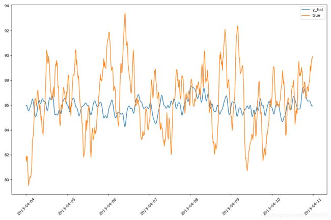
从下图可以看出，prophet预测值是跟这个arma过程的收敛值一致，也就是说近乎用一个常数来预测该arma序列；该arma模型的收敛点是 85.79985020557761，如图所示，prophet的预测值几乎跟这个值一致；

2.3 生成一个带趋势的时间序列

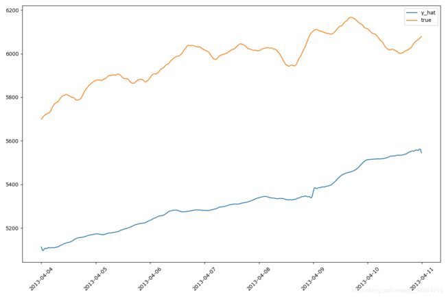
仍然以案例二中的时间序列为例，这次我们将arma过程变换成一个带趋势的过程，可以直接添加一个时间t的函数，也可以直接将案例2中的arma数据相加，为了演示方便，我们将趋势项调小，即将案例二中的constant参数调整为0.1，此时生成的数据如下：

arima_model_object = arima_model(Constant=0.1, AR={1:0.47,2:0.39}, MA={1:1.0,2:0.7,3:0.4}, Variance=0.5)
simulate_samples = 96*100
simulate_y = arima_model_object.simulate(simulate_samples)
print(simulate_y.__len__())
scale_mean = simulate_y.mean()
scale_std = simulate_y.std()
print("mean:",scale_mean)
print("std:",scale_std)



# x = np.arange(0,1000,1/50)
dates = pd.date_range(start='20130101', periods=len(simulate_y), freq="15min")
# 平稳
# y = simulate_y
# 非平稳
y = np.cumsum(simulate_y)
df = pd.DataFrame(y[0:len(dates)], index=dates).reset_index()
df.rename(columns={0: "y", "index": "ds"}, inplace=True)
df_train = df[df.ds < '2013-04-04']
df_test = df[df.ds >= '2013-04-04']

plt.figure(1, figsize=(12, 8))
plt.plot(df["ds"],df["y"])
plt.xticks(rotation=45)
plt.show()

3.总结

• 当时间序列含有固定周期成分，利用prophet可以较好的估计周期成分；但是需要正确的设置周期的大小和相应的傅里叶级数项数；
• 当数据的生成过程是arma时，propeht基本上是按照arma模型的均值来预测，对于arma类的数据生成过程，这种预测是合理的；
• 当生成非平稳的时间序列时，发现prophet在不调参的情况下，并没有精确的预测数据的走势，一方面由于我们生成的时间序列中的不确定性成分占比较高，另一方面，我们也没有做参数优化，达到目前的预测精度，是能接受的。